Survey Analysis¶

We often want to survey people on their views or reactions to possible events (design or promotion, for example). There are many survey tools that are good in designing the survey, presenting it on various forms, such as web or mobile, distributing it and collecting the responses. However, when it comes to analyzing the responses, you are left with fewer options, and most of them are out-dated (SPSS, for example).

In this notebook, we will explore how to analyze survey’s responses, including statistical tests for reliability and research hypothesis.

We will start with loading the CSV files that we exported from the survey system (Qualtrics, in this example).

import warnings
warnings.filterwarnings('ignore')

import pandas as pd

survey_df = pd.read_csv('../data/survey_results.csv')

Survery Overview¶

We can explore the number of questions and answers with info

survey_df.info()

<class 'pandas.core.frame.DataFrame'>
RangeIndex: 97 entries, 0 to 96
Data columns (total 65 columns):
 #   Column                 Non-Null Count  Dtype 
---  ------                 --------------  ----- 
 StartDate              97 non-null     object
 EndDate                97 non-null     object
 Status                 97 non-null     object
 IPAddress              97 non-null     object
 Progress               97 non-null     object
 Duration (in seconds)  97 non-null     object
 Finished               97 non-null     object
 RecordedDate           97 non-null     object
 ResponseId             97 non-null     object
 RecipientLastName      1 non-null      object
RecipientFirstName     1 non-null      object
RecipientEmail         1 non-null      object
ExternalReference      1 non-null      object
LocationLatitude       97 non-null     object
LocationLongitude      97 non-null     object
DistributionChannel    97 non-null     object
UserLanguage           97 non-null     object
Q_RecaptchaScore       95 non-null     object
E1                     97 non-null     object
A2                     97 non-null     object
C3                     97 non-null     object
N4                     97 non-null     object
I5                     97 non-null     object
E6R                    97 non-null     object
A7R                    97 non-null     object
C8R                    97 non-null     object
N9R                    97 non-null     object
I10R                   97 non-null     object
E11                    97 non-null     object
A12                    97 non-null     object
C13                    97 non-null     object
N14                    97 non-null     object
I15R                   97 non-null     object
E16R                   97 non-null     object
A17R                   97 non-null     object
C18R                   97 non-null     object
N19R                   97 non-null     object
I20R                   97 non-null     object
Q71_First Click        50 non-null     object
Q71_Last Click         50 non-null     object
Q71_Page Submit        50 non-null     object
Q71_Click Count        50 non-null     object
Q73_First Click        48 non-null     object
Q73_Last Click         48 non-null     object
Q73_Page Submit        48 non-null     object
Q73_Click Count        48 non-null     object
Expectation1           97 non-null     object
Expectation2           97 non-null     object
Trust1                 97 non-null     object
Trust2                 97 non-null     object
Trust5                 97 non-null     object
Trust6                 97 non-null     object
Trust7                 97 non-null     object
Trust8                 97 non-null     object
Trust9                 97 non-null     object
Expectation3           97 non-null     object
Offering1              97 non-null     object
Offering2              97 non-null     object
Offering3              97 non-null     object
Gender                 97 non-null     object
Age                    97 non-null     object
Education              97 non-null     object
Region                 97 non-null     object
Q53                    97 non-null     object
Random ID              97 non-null     object
dtypes: object(65)
memory usage: 49.4+ KB

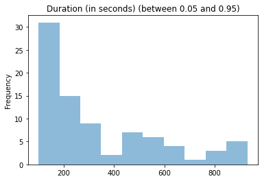
Cliping outliers¶

We want to remove outliers to avoid issues from people answering too quick or too slow. Let’s calculate the 0.05 and 0.95 percentiles of the data:

(
    survey_df
    .loc[1:,['Duration (in seconds)']]
    .astype(int)
    .quantile([0.05, 0.95])
)

	Duration (in seconds)
0.05	87.25
0.95	1171.00

And now we can clip the data to be above 90 and below 1,100

valid_survey_df = (
    survey_df
    .loc[1:,:]
    .assign(duration = lambda x : pd.to_numeric(x['Duration (in seconds)']))
    .query("duration > 90 and duration < 1100")
)
valid_survey_df

	StartDate	EndDate	Status	IPAddress	Progress	Duration (in seconds)	Finished	RecordedDate	ResponseId	RecipientLastName	...	Offering1	Offering2	Offering3	Gender	Age	Education	Region	Q53	Random ID	duration
1	2/19/2021 3:28:19	2/19/2021 3:30:28	IP Address	47.35.194.33	100	129	True	2/19/2021 3:30:29	R_2WUYft76PXR2zBS	NaN	...	3	4	2	Female	40-50	Bachelor’s degree	North America	IM_6m0pkPqaVoiPxY1	58834	129
2	2/19/2021 3:28:16	2/19/2021 3:30:36	IP Address	151.65.216.111	100	140	True	2/19/2021 3:30:37	R_3eq8jucMfNqn5A4	NaN	...	5	5	3	Male	18-28	Bachelor’s degree	Europe	IM_6m0pkPqaVoiPxY1	21882	140
3	2/19/2021 3:29:12	2/19/2021 3:31:01	IP Address	73.176.57.130	100	108	True	2/19/2021 3:31:01	R_1jOnl4rE5r7qMcE	NaN	...	Very likely\n7	6	6	Male	29-39	Bachelor’s degree	North America	IM_6m0pkPqaVoiPxY1	59587	108
4	2/19/2021 3:29:18	2/19/2021 3:31:07	IP Address	86.106.87.89	100	109	True	2/19/2021 3:31:07	R_BxBBo8wdgckIP7j	NaN	...	4	5	Very influential\n7	Male	29-39	Bachelor’s degree	South America	IM_6m0pkPqaVoiPxY1	52402	109
5	2/19/2021 3:29:06	2/19/2021 3:31:28	IP Address	27.57.12.252	100	142	True	2/19/2021 3:31:29	R_2ea55lhudZuzX2J	NaN	...	5	5	4	Male	29-39	Master Degree	Asia	IM_6m0pkPqaVoiPxY1	64888	142
...	...	...	...	...	...	...	...	...	...	...	...	...	...	...	...	...	...	...	...	...	...
92	2/19/2021 4:01:13	2/19/2021 4:15:24	IP Address	117.199.129.182	100	850	True	2/19/2021 4:15:24	R_3HXHwga41cOCWJ3	NaN	...	6	5	Very influential\n7	Female	29-39	Bachelor’s degree	Asia	IM_6m0pkPqaVoiPxY1	23065	850
93	2/19/2021 4:05:50	2/19/2021 4:15:54	IP Address	196.18.164.102	100	604	True	2/19/2021 4:15:55	R_2sTpV27TMoq55Nj	NaN	...	5	5	5	Female	+62	Bachelor’s degree	North America	IM_6m0pkPqaVoiPxY1	56488	604
94	2/19/2021 4:14:37	2/19/2021 4:17:39	IP Address	70.39.92.10	100	181	True	2/19/2021 4:17:39	R_10IT3z1yGSWIddU	NaN	...	Very likely\n7	Very probable\n7	Very influential\n7	Female	29-39	Bachelor’s degree	North America	IM_6m0pkPqaVoiPxY1	10094	181
95	2/19/2021 4:10:47	2/19/2021 4:18:35	IP Address	182.65.119.175	100	467	True	2/19/2021 4:18:35	R_2q9815sUara9kKO	NaN	...	6	Very probable\n7	Very influential\n7	Female	29-39	Master Degree	Asia	IM_6m0pkPqaVoiPxY1	88800	467
96	2/19/2021 4:20:30	2/19/2021 4:22:18	IP Address	117.213.34.183	100	108	True	2/19/2021 4:22:19	R_2VpU6ciTRw7Kdyf	NaN	...	5	Very probable\n7	6	Male	29-39	Bachelor’s degree	Asia	IM_6m0pkPqaVoiPxY1	68054	108

83 rows × 66 columns

(
    valid_survey_df
    ['duration']
    .plot(
        kind='hist', 
        alpha=0.5, 
        title='Duration (in seconds) (between 0.05 and 0.95)'
    )
);

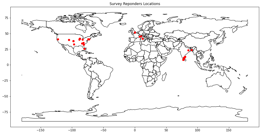
../_images/08.04_Survey_analysis_10_0.png

Map of responders¶

Most of the survey tools are also reporting regarding the location of the responders with their location information. This survey also has this data in LocationLongitude and Locationlatitude columns. We can use the popular GeoPandas package to show them over the world map.

Create from GeoPandas
a geo-location data frame
based on the survey table above
Use the geometry information to draw points based on
\(x\) as location longitude, and
\(y\) as location latitude

%pip install geopandas --quiet

Note: you may need to restart the kernel to use updated packages.

import geopandas
import matplotlib.pyplot as plt

gdf = (
    geopandas
    .GeoDataFrame(
        valid_survey_df, 
        geometry=geopandas.points_from_xy(
            valid_survey_df.LocationLongitude, 
            valid_survey_df.LocationLatitude)
        )
)

Create a map of the world based on the built-in map from GeoPandas
Plot the background map with
while background and
black lines
and the locations of the responders in red
Set the title of the map to “Survey Reponders Locations”

world = (
    geopandas
    .read_file(
        geopandas
        .datasets
        .get_path('naturalearth_lowres')
    )
)

gdf.plot(
    ax=(
        world
        .plot(
            color='white', 
            edgecolor='black',
            figsize=(15,10)
        )
    ), 
    color='red',
    
).set_title("Survey Reponders Locations");

../_images/08.04_Survey_analysis_15_0.png

Personality Score¶

The first part of the survey was a personality score that we need to analyze to build the score of each responder. We can find the psychology test format in a previous reserach:

Mini-IPIP test questions¶

Based on: “The Mini-IPIP Scales: Tiny-Yet-Effective Measures of the Big Five Factors of Personality”

Appendix 20-Item Mini-IPIP

Item	Factor	Text
1	E	Am the life of the party.
2	A	Sympathize with others’ feelings
3	C	Get chores done right away.
4	N	Have frequent mood swings.
5	I	Have a vivid imagination.
6	E	Don’t talk a lot. (R)
7	A	Am not interested in other people’s problems. (R)
8	C	Often forget to put things back in their proper place. (R)
9	N	Am relaxed most of the time. (R)
10	I	Am not interested in abstract ideas. (R)
11	E	Talk to a lot of different people at parties.
12	A	Feel others’ emotions.
13	C	Like order.
14	N	Get upset easily.
15	I	Have difficulty understanding abstract ideas. (R)
16	E	Keep in the background. (R)
17	A	Am not really interested in others. (R)
18	C	Make a mess of things. (R)
19	N	Seldom feel blue. (R)
20	I	Do not have a good imagination. (R)

First, let’s get the questions that are written in the first line (index=0) of the table. We want the 20 questions from index 18 to index 38.

(
    survey_df
    .iloc[0,18:38]
)

E1                              Am the life of the party.
A2                      Sympathize with others' feelings.
C3                            Get chores done right away.
N4                             Have frequent mood swings.
I5                              Have a vivid imagination.
E6R                                     Don't talk a lot.
A7R         Am not interested in other people's problems.
C8R     Often forget to put things back in their prope...
N9R                          Am relaxed most of the time.
I10R                 Am not interested in abstract ideas.
E11         Talk to a lot of different people at parties.
A12                                Feel others' emotions.
C13                                           Like order.
N14                                     Get upset easily.
I15R        Have difficulty understanding abstract ideas.
E16R                              Keep in the background.
A17R                  Am not really interested in others.
C18R                               Make a mess of things.
N19R                                    Seldom feel blue.
I20R                      Do not have a good imagination.
Name: 0, dtype: object

Let’s check how the results look like in the table:

survey_df.E1

   Am the life of the party.
        Strongly Disagree\n1
        Strongly Disagree\n1
           Somewhat agree\n4
           Somewhat agree\n4
                ...            
          Somewhat agree\n4
       Strongly Disagree\n1
          Somewhat agree\n4
       Strongly Disagree\n1
          Strongly agree\n5
Name: E1, Length: 97, dtype: object

We see that we have five personality traits that we are measuring with these questions: E, A, C, N, I.

Create a variable for each personality trait above
Convert each question to its relevant trait by taking the numertic score at the last character of the question as an Integer, and add it to the relevant trait score. Note that some of the scores are reversed and you need to add the reversed score (6 - score, for a 1-5 score as we have here)

survey_ipip_df = (
    valid_survey_df
    # Initial values to 0
    .assign(E = 0)
    .assign(A = 0)
    .assign(C = 0)
    .assign(N = 0)
    .assign(I = 0)
    # Update based on survy score
    .assign(E = lambda x : x.E + x.E1.str[-1:].astype(int))
    .assign(A = lambda x : x.A + x.A2.str[-1:].astype(int))
    .assign(C = lambda x : x.C + x.C3.str[-1:].astype(int))
    .assign(N = lambda x : x.N + x.N4.str[-1:].astype(int))
    .assign(I = lambda x : x.I + x.I5.str[-1:].astype(int))
    .assign(E = lambda x : x.E + 6 - x.E6R.str[-1:].astype(int))
    .assign(A = lambda x : x.A + 6 - x.A7R.str[-1:].astype(int))
    .assign(C = lambda x : x.C + 6 - x.C8R.str[-1:].astype(int))
    .assign(N = lambda x : x.N + 6 - x.N9R.str[-1:].astype(int))
    .assign(I = lambda x : x.I + 6 - x.I10R.str[-1:].astype(int))
    .assign(E = lambda x : x.E + x.E11.str[-1:].astype(int))
    .assign(A = lambda x : x.A + x.A12.str[-1:].astype(int))
    .assign(C = lambda x : x.C + x.C13.str[-1:].astype(int))
    .assign(N = lambda x : x.N + x.N14.str[-1:].astype(int))
    .assign(I = lambda x : x.I + 6 - x.I15R.str[-1:].astype(int))
    .assign(E = lambda x : x.E + 6 - x.E16R.str[-1:].astype(int))
    .assign(A = lambda x : x.A + 6 - x.A17R.str[-1:].astype(int))
    .assign(C = lambda x : x.C + 6 - x.C18R.str[-1:].astype(int))
    .assign(N = lambda x : x.N + 6 - x.N19R.str[-1:].astype(int))
    .assign(I = lambda x : x.I + 6 - x.I20R.str[-1:].astype(int))
    # Calculate the average
    .assign(E = lambda x : x.E / 4)
    .assign(A = lambda x : x.A / 4)
    .assign(C = lambda x : x.C / 4)
    .assign(N = lambda x : x.N / 4)
    .assign(I = lambda x : x.I / 4)
)

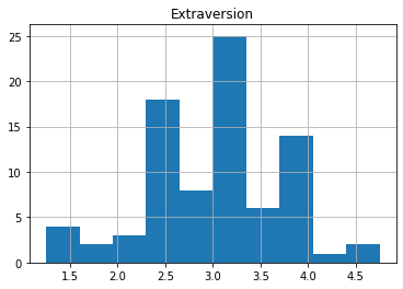
Personality Trait Visualization¶

We can show a quick histogram of one or two of the traits

(
    survey_ipip_df
    .E
    .hist()
).set_title("Extraversion");

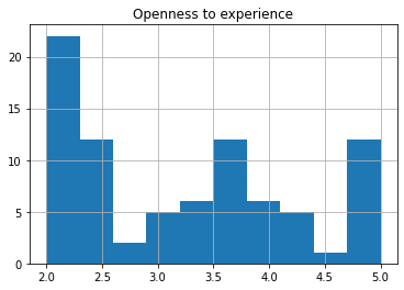
../_images/08.04_Survey_analysis_25_0.png

(
    survey_ipip_df
    .I
    .hist()
).set_title("Openness to experience");

../_images/08.04_Survey_analysis_26_0.png

Random Groups¶

Many tests are using split to random groups to check the effect of a treatment on one of the group, while using the other group as a control group (or any other similar test method). In the survey, the group will be visible with answers on some of the questions, while other groups will answer different questions. In this survey, there were two groups that were assigned randomaly question 71 or question 73.

Create a new column in the table called group
create the first condition to have an answer (not null) in Q71 column
create the second condition to have an answer in Q73 column
assign the group value to be ‘Group A’ for the first condition
assign the group value to be ‘Group B’ for the second condition
assign a default value ‘Unknown’ if none of the condition is mapped

import numpy as np
survey_ipip_df['group'] = np.select(
    [
        survey_ipip_df['Q71_Page Submit'].notnull(), 
        survey_ipip_df['Q73_Page Submit'].notnull(), 
    ], 
    [
        'Group A', 
        'Group B'
    ], 
    default='Unknown'
)

Research questions¶

The third part is the research questions part, where we want to test the impact of the treatment on the answers to these questions. From the list of columns in the table that we did in the beginning we see that these are starting with ‘Expectation1’, and ends with ‘Offering3’

survey_questions = (
    survey_df
    .loc[0,'Expectation1':'Offering3']
)
survey_questions

Expectation1          The chatbot's messages met my expectations.
Expectation2    The chatbot's messages corresponded to how I e...
Trust1                  The bike chatbot seemed to care about me.
Trust2                        The bike chatbot made me feel good.
Trust5             I believe the bike chatbot was honest with me.
Trust6          I believe the bike chatbot didn’t make false c...
Trust7                 I believe the bike chatbot is trustworthy.
Trust8                                  I trust the bike chatbot.
Trust9              The bike chatbot seemed adequate to my needs.
Expectation3             The chatbot's messages were appropriate.
Offering1       What is the likelihood that you would accept t...
Offering2       How probable is it that you would accept the c...
Offering3       How influential do you perceive the chatbot’s ...
Name: 0, dtype: object

Convert all the values of these questions to numeric values based on the last characters ([-1:]) of the answer and set its type to be Interger

numeric_survey_ipip_df = (
    survey_ipip_df
    .apply(lambda x: 
        x.str[-1:].astype(int) 
        if x.name.startswith('Expectation') 
        else x
    )
    .apply(lambda x: 
        x.str[-1:].astype(int) 
        if x.name.startswith('Trust') 
        else x
    )
    .apply(lambda x: 
        x.str[-1:].astype(int) 
        if x.name.startswith('Offering') 
        else x
    )
)

Testing Reliability with Cronbach’s \(\alpha\)¶

A common test to check the reliability of the answers is to test them using Cronbach’s alpha test. We expect that all the questions that are related to Trust, for example, will have a high correlation, and therefore a cronbach-alpha score that is higher than 0.7.

First, let’s install a python library with cronbach-alpha function in it.

pip install pingouin --quiet

Note: you may need to restart the kernel to use updated packages.

import pingouin as pg

Now, let’s take the set of questions for each variable (Expectation, Trust, and Offering in this survey) and calculate their score:

pg.cronbach_alpha(data=
    numeric_survey_ipip_df
    .loc[:,
        ['Expectation1','Expectation2','Expectation3']
    ]
)

(0.7635463917525775, array([0.659, 0.84 ]))

pg.cronbach_alpha(data=
    numeric_survey_ipip_df
    .loc[:,
        ['Trust1','Trust2','Trust5','Trust6','Trust7','Trust8','Trust9']
    ]
)

(0.7665523059220511, array([0.681, 0.836]))

pg.cronbach_alpha(data=
    numeric_survey_ipip_df
    .loc[:,
        ['Offering1','Offering2','Offering3']
    ]
)

(0.7863454562366294, array([0.692, 0.855]))

Calculate the research variables¶

Now that we see that the reliability of the question is good enough (>0.7), we can calculate the average score of each of these questions sets. We will use eval function to do it:

summary_numeric_survey_df = (
    numeric_survey_ipip_df
    .eval("Expectation = (Expectation1 + Expectation2 + Expectation3) / 3")
    .eval("Offering = (Offering1 + Offering2 + Offering3) / 3")
    .eval("Trust = (Trust1 + Trust2 + Trust5 + Trust6 + Trust7 + Trust8 + Trust9) / 7")
)

(
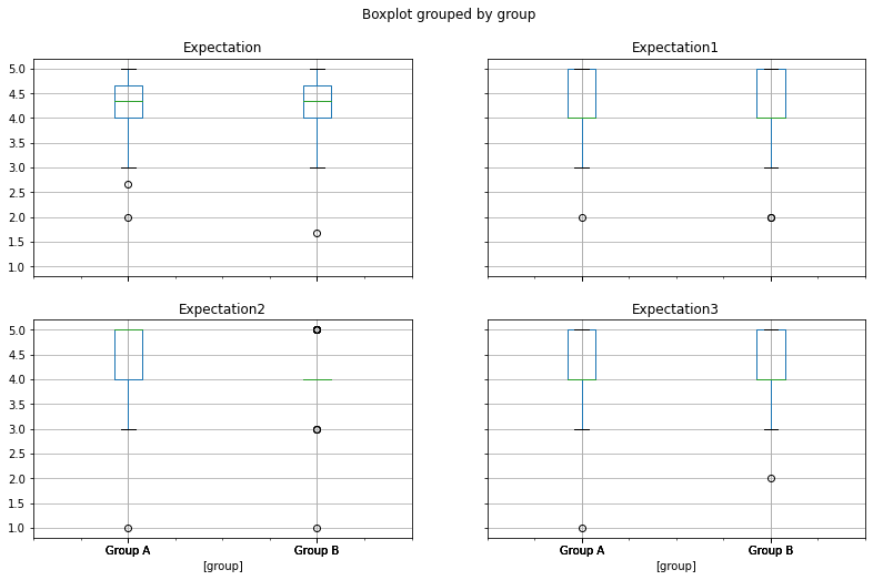
    summary_numeric_survey_df
    [['Expectation','Expectation1','Expectation2','Expectation3','group']]
    .boxplot(by='group', figsize=(13,8))
);

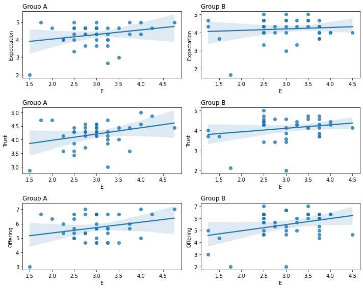
../_images/08.04_Survey_analysis_43_0.png

We can plot the correlation of any of the personality traits (first part of the survey), with the score to any of the research questions (third part), within the two different grups (second part)

Create a grid of 3 by 2 to show the graphs of the research question * groups
For each one of the reserach questions and
for each of the groups
filter the table to include only the current group
Plot a regression plot (points, line and confidence area)
\(x\) as E (personality)
\(y\) as the research question
on the chart grid
Set the title of each graph the name of the group

import seaborn as sns
### PLOT BUILD
fig, ax = plt.subplots(3, 2, figsize=(10,8))

for idx, attribute in enumerate(['Expectation','Trust','Offering']):
    for i, group in enumerate(['Group A', 'Group B']):
        sub_df = (
            summary_numeric_survey_df
            .query('group == @group')
        )
        (
            sns
            .regplot(
                x=sub_df.E, 
                y=sub_df[attribute], 
                ax=ax[idx,i]
            )
        )
        ax[idx,i].set_title(group, loc='left')
fig.tight_layout()

plt.show()

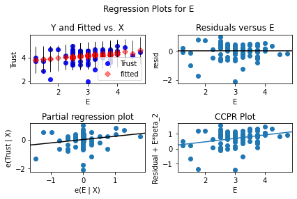
../_images/08.04_Survey_analysis_45_0.png

Anova¶

The last part of the analysis is the null hypothsis check that the groups are making a different impact on the relationship between the personality trait and the reserach questions.

import statsmodels.api as sm
from statsmodels.formula.api import ols

model = ols(
        f'Trust ~ C(group) * E', 
        data=(
            summary_numeric_survey_df
            .loc[:,['E','Trust','group']]
        )
    ).fit()
fig = sm.graphics.plot_regress_exog(model, "E")
fig.tight_layout(pad=1.0)

eval_env: 1

../_images/08.04_Survey_analysis_48_1.png

for attribute in ['Expectation','Trust','Offering']:
    print(attribute)
    model = ols(
        f'{attribute} ~ C(group) * E', 
        data=(
            summary_numeric_survey_df
            .loc[:,['E',attribute,'group']]
        )
    ).fit()
    display(model.summary())
    anova_table = sm.stats.anova_lm(model, typ=2)
    display(anova_table)
    display(summary_numeric_survey_df.anova(dv=attribute, between=['group','E']).round(3))

Expectation

OLS Regression Results
Dep. Variable:	Expectation	R-squared:	0.045
Model:	OLS	Adj. R-squared:	0.009
Method:	Least Squares	F-statistic:	1.240
Date:	Sun, 22 May 2022	Prob (F-statistic):	0.301
Time:	20:29:15	Log-Likelihood:	-76.904
No. Observations:	83	AIC:	161.8
Df Residuals:	79	BIC:	171.5
Df Model:	3
Covariance Type:	nonrobust

	coef	std err	t	P>\|t\|	[0.025	0.975]
Intercept	3.5115	0.471	7.453	0.000	2.574	4.449
C(group)[T.Group B]	0.4466	0.619	0.721	0.473	-0.786	1.680
E	0.2620	0.155	1.695	0.094	-0.046	0.570
C(group)[T.Group B]:E	-0.1816	0.202	-0.897	0.372	-0.584	0.221

Omnibus:	32.242	Durbin-Watson:	2.149
Prob(Omnibus):	0.000	Jarque-Bera (JB):	61.305
Skew:	-1.480	Prob(JB):	4.87e-14
Kurtosis:	5.995	Cond. No.	41.4

Notes:
[1] Standard Errors assume that the covariance matrix of the errors is correctly specified.

	sum_sq	df	F	PR(>F)
C(group)	0.188292	1.0	0.479798	0.490545
E	0.960168	1.0	2.446659	0.121772
C(group):E	0.315844	1.0	0.804820	0.372382
Residual	31.002798	79.0	NaN	NaN

/opt/hostedtoolcache/Python/3.7.13/x64/lib/python3.7/site-packages/statsmodels/base/model.py:1873: ValueWarning: covariance of constraints does not have full rank. The number of constraints is 14, but rank is 10
  'rank is %d' % (J, J_), ValueWarning)

	Source	SS	DF	MS	F	p-unc	np2
0	group	2.738	1.0	2.738	10.734	0.002	0.154
1	E	2069.063	14.0	147.790	579.413	0.000	0.993
2	group * E	35.160	14.0	2.511	9.846	0.000	0.700
3	Residual	15.049	59.0	0.255	NaN	NaN	NaN

Trust

OLS Regression Results
Dep. Variable:	Trust	R-squared:	0.076
Model:	OLS	Adj. R-squared:	0.041
Method:	Least Squares	F-statistic:	2.173
Date:	Sun, 22 May 2022	Prob (F-statistic):	0.0978
Time:	20:29:15	Log-Likelihood:	-61.619
No. Observations:	83	AIC:	131.2
Df Residuals:	79	BIC:	140.9
Df Model:	3
Covariance Type:	nonrobust

	coef	std err	t	P>\|t\|	[0.025	0.975]
Intercept	3.5102	0.392	8.956	0.000	2.730	4.290
C(group)[T.Group B]	0.0700	0.515	0.136	0.892	-0.956	1.096
E	0.2309	0.129	1.796	0.076	-0.025	0.487
C(group)[T.Group B]:E	-0.0562	0.168	-0.334	0.739	-0.391	0.279

Omnibus:	34.337	Durbin-Watson:	1.722
Prob(Omnibus):	0.000	Jarque-Bera (JB):	75.187
Skew:	-1.487	Prob(JB):	4.71e-17
Kurtosis:	6.591	Cond. No.	41.4

Notes:
[1] Standard Errors assume that the covariance matrix of the errors is correctly specified.

	sum_sq	df	F	PR(>F)
C(group)	0.198562	1.0	0.731283	0.395054
E	1.546282	1.0	5.694801	0.019408
C(group):E	0.030313	1.0	0.111641	0.739169
Residual	21.450497	79.0	NaN	NaN

/opt/hostedtoolcache/Python/3.7.13/x64/lib/python3.7/site-packages/statsmodels/base/model.py:1873: ValueWarning: covariance of constraints does not have full rank. The number of constraints is 14, but rank is 10
  'rank is %d' % (J, J_), ValueWarning)

	Source	SS	DF	MS	F	p-unc	np2
0	group	2.673	1.0	2.673	14.043	0.0	0.192
1	E	1980.174	14.0	141.441	743.184	0.0	0.994
2	group * E	26.872	14.0	1.919	10.085	0.0	0.705
3	Residual	11.229	59.0	0.190	NaN	NaN	NaN

Offering

OLS Regression Results
Dep. Variable:	Offering	R-squared:	0.111
Model:	OLS	Adj. R-squared:	0.077
Method:	Least Squares	F-statistic:	3.291
Date:	Sun, 22 May 2022	Prob (F-statistic):	0.0249
Time:	20:29:15	Log-Likelihood:	-114.53
No. Observations:	83	AIC:	237.1
Df Residuals:	79	BIC:	246.7
Df Model:	3
Covariance Type:	nonrobust

	coef	std err	t	P>\|t\|	[0.025	0.975]
Intercept	4.5893	0.741	6.190	0.000	3.114	6.065
C(group)[T.Group B]	-0.6425	0.975	-0.659	0.512	-2.583	1.298
E	0.3777	0.243	1.553	0.124	-0.106	0.862
C(group)[T.Group B]:E	0.1288	0.318	0.404	0.687	-0.505	0.763

Omnibus:	14.535	Durbin-Watson:	1.891
Prob(Omnibus):	0.001	Jarque-Bera (JB):	16.718
Skew:	-0.898	Prob(JB):	0.000234
Kurtosis:	4.267	Cond. No.	41.4

Notes:
[1] Standard Errors assume that the covariance matrix of the errors is correctly specified.

	sum_sq	df	F	PR(>F)
C(group)	1.381213	1.0	1.421506	0.236725
E	8.083278	1.0	8.319086	0.005054
C(group):E	0.158976	1.0	0.163614	0.686944
Residual	76.760714	79.0	NaN	NaN

/opt/hostedtoolcache/Python/3.7.13/x64/lib/python3.7/site-packages/statsmodels/base/model.py:1873: ValueWarning: covariance of constraints does not have full rank. The number of constraints is 14, but rank is 10
  'rank is %d' % (J, J_), ValueWarning)

	Source	SS	DF	MS	F	p-unc	np2
0	group	9.509	1.0	9.509	11.908	0.001	0.168
1	E	3593.710	14.0	256.694	321.460	0.000	0.987
2	group * E	62.507	14.0	4.465	5.591	0.000	0.570
3	Residual	47.113	59.0	0.799	NaN	NaN	NaN

Another way to calculate Anova One Way¶

import scipy.stats as stats

fvalue, pvalue = (
    stats
    .f_oneway(
        summary_numeric_survey_df['E'],
        summary_numeric_survey_df['Trust']
    )
)
print(fvalue, pvalue)

147.41775587209213 1.3074590620296686e-24

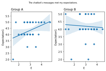
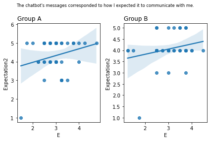
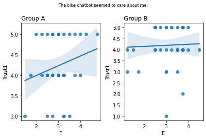
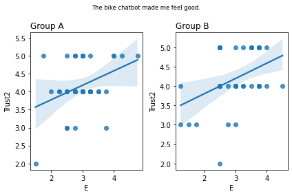
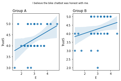
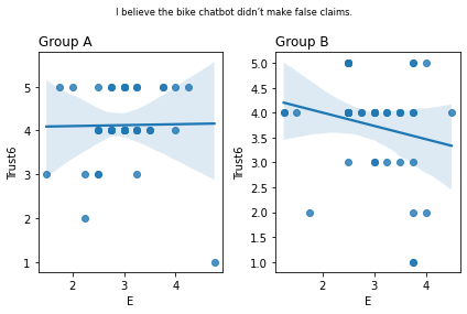
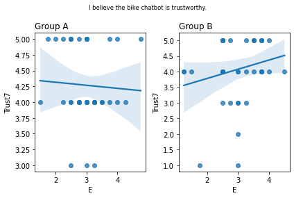
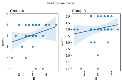
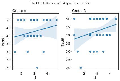
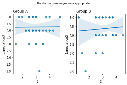
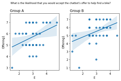
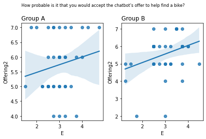
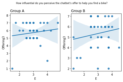
Graphs of all questions¶

for q_num, q in survey_questions.iteritems():
    fig, ax = plt.subplots(1, 2)

    for i,group in enumerate(sorted(summary_numeric_survey_df.group.unique())):
        sub_df = (
            summary_numeric_survey_df
            .query('group == @group')
        )
        (
            sns
            .regplot(
                x=sub_df['E'], 
                y=sub_df[q_num], 
                ax=ax[i]
            )
        )
        ax[i].set_title(group, loc='left')

    fig.suptitle(q, fontsize='small')
    fig.tight_layout()

    plt.show()

../_images/08.04_Survey_analysis_53_0.png

../_images/08.04_Survey_analysis_53_1.png

../_images/08.04_Survey_analysis_53_2.png

../_images/08.04_Survey_analysis_53_3.png

../_images/08.04_Survey_analysis_53_4.png

../_images/08.04_Survey_analysis_53_5.png

../_images/08.04_Survey_analysis_53_6.png

../_images/08.04_Survey_analysis_53_7.png

../_images/08.04_Survey_analysis_53_8.png

../_images/08.04_Survey_analysis_53_9.png

../_images/08.04_Survey_analysis_53_10.png

../_images/08.04_Survey_analysis_53_11.png

../_images/08.04_Survey_analysis_53_12.png

from scipy.stats import spearmanr
for q_num, q in survey_questions.iteritems():
    stat, p = spearmanr(
        (
            summary_numeric_survey_df
            .query('group == "Group A"')
            .iloc[:41,:]
            [q_num]
        ),
        (
            summary_numeric_survey_df
            .query('group == "Group B"')
            .iloc[:41,:]
            [q_num]
        )
    )
    print('stat=%.3f, p=%.3f' % (stat, p),q)

stat=0.346, p=0.027 The chatbot's messages met my expectations.
stat=0.342, p=0.029 The chatbot's messages corresponded to how I expected it to communicate with me.
stat=0.197, p=0.216 The bike chatbot seemed to care about me.
stat=0.117, p=0.467 The bike chatbot made me feel good.
stat=0.036, p=0.823 I believe the bike chatbot was honest with me.
stat=0.068, p=0.675 I believe the bike chatbot didn’t make false claims.
stat=0.139, p=0.385 I believe the bike chatbot is trustworthy.
stat=0.119, p=0.459 I trust the bike chatbot.
stat=0.292, p=0.064 The bike chatbot seemed adequate to my needs.
stat=0.008, p=0.963 The chatbot's messages were appropriate.
stat=0.029, p=0.855 What is the likelihood that you would accept the chatbot’s offer to help find a bike?
stat=0.029, p=0.856 How probable is it that you would accept the chatbot’s offer to help find a bike?
stat=0.126, p=0.434 How influential do you perceive the chatbot’s offer to help you find a bike?

SPSS Files¶

Pandas can also load SPSS files

#pip install pyreadstat

#spss_df = pd.read_spss()

#spss_df

From Excel to Pandas

Survey Analysis

Contents

Survey Analysis¶

Survery Overview¶

Cliping outliers¶

Map of responders¶

Personality Score¶

Mini-IPIP test questions¶

Personality Trait Visualization¶

Random Groups¶

Research questions¶

Testing Reliability with Cronbach’s \(\alpha\)¶

Calculate the research variables¶

Anova¶

Another way to calculate Anova One Way¶

Graphs of all questions¶

SPSS Files¶