Currency Rate Analysis¶

Money often costs too much. –Ralph Waldo Emerson

A very used expression in our life, and if utilized just right, also very useful.

In this notebook, we query a REST API to get the latest currency rates for many currencies. Using dynamic API compared to loading static files allows for updated data to be processed.

We will start with removing code warnings to make it easier to read the notebook.

import warnings
warnings.filterwarnings('ignore')

Loading data using API¶

First of all, let’s get our data.

In order to do so, let’s start with installing all the needed libraries and get the right imports.

%pip install forex-python --quiet

Note: you may need to restart the kernel to use updated packages.

import pandas as pd
import numpy as np

from forex_python.converter import CurrencyRates
from datetime import datetime

Let’s get the data

In that case, the function here is given by the provider of this API, and for more methods, you can go to forext-python usage page

usd_rates = (
    CurrencyRates()
    .get_rates('USD')
)
usd_rates

{'EUR': 0.9454476694714947,
 'JPY': 127.95688758627209,
 'BGN': 1.8491065519523493,
 'CZK': 23.324194005861774,
 'DKK': 7.036399735274652,
 'GBP': 0.8019287132457218,
 'HUF': 362.0402760707195,
 'PLN': 4.383568119504585,
 'RON': 4.6777914342441145,
 'SEK': 9.919164224260186,
 'CHF': 0.9719202042166966,
 'ISK': 130.94450222180203,
 'NOK': 9.702183984116479,
 'HRK': 7.122530017963506,
 'TRY': 15.902524345277488,
 'AUD': 1.416280608868299,
 'BRL': 4.915287888815354,
 'CAD': 1.2788125177271437,
 'CNY': 6.678453247612744,
 'HKD': 7.847121111846458,
 'IDR': 14656.320317670416,
 'INR': 77.6795877848161,
 'KRW': 1267.4482367400963,
 'MXN': 19.884088115722793,
 'MYR': 4.388957171220572,
 'NZD': 1.5616904604330148,
 'PHP': 52.17074784910655,
 'SGD': 1.3792190602250165,
 'THB': 34.30462323910371,
 'ZAR': 15.801361444644039}

Let’s turn it into something more readable and easier to manipulate, by converting its type from Dictionary to DataFrame, and give its columns proper informative names.

usd_rates_df = (
    pd
    .DataFrame
    .from_dict(usd_rates, orient='index')
    .rename(columns={0 : 'Rate'})
)
usd_rates_df

	Rate
EUR	0.945448
JPY	127.956888
BGN	1.849107
CZK	23.324194
DKK	7.036400
GBP	0.801929
HUF	362.040276
PLN	4.383568
RON	4.677791
SEK	9.919164
CHF	0.971920
ISK	130.944502
NOK	9.702184
HRK	7.122530
TRY	15.902524
AUD	1.416281
BRL	4.915288
CAD	1.278813
CNY	6.678453
HKD	7.847121
IDR	14656.320318
INR	77.679588
KRW	1267.448237
MXN	19.884088
MYR	4.388957
NZD	1.561690
PHP	52.170748
SGD	1.379219
THB	34.304623
ZAR	15.801361

This looks like a useful table to have if you work with multiple currencies in your organization

Getting rates for a specific date¶

We will use the date functionality from the API provider.

Call the currency API
Request exchange rates
for USD
for 2020-05-23

usd_rate_on_date = (
   CurrencyRates()
    .get_rates(
        'USD',
        datetime(2020, 5, 23)
    )
)
usd_rate_on_date

{'EUR': 0.917094644167278,
 'USD': 1,
 'JPY': 107.53851797505503,
 'BGN': 1.7936537050623624,
 'CZK': 24.954145267791635,
 'DKK': 6.839508437270726,
 'GBP': 0.8213774761555392,
 'HUF': 320.43286867204694,
 'PLN': 4.146093176815848,
 'RON': 4.44194790902421,
 'SEK': 9.663701393983859,
 'CHF': 0.9712949376375641,
 'ISK': 143.34189288334557,
 'NOK': 10.003484959647835,
 'HRK': 6.95570432868672,
 'RUB': 71.45442039618489,
 'TRY': 6.807318415260455,
 'AUD': 1.530997798972854,
 'BRL': 5.581162876008804,
 'CAD': 1.400678650036684,
 'CNY': 7.134721203228173,
 'HKD': 7.7559611151870875,
 'IDR': 14901.999266324283,
 'ILS': 3.5270542920029344,
 'INR': 75.86803008070433,
 'KRW': 1241.2967718268526,
 'MXN': 22.96863536316948,
 'MYR': 4.362527512839325,
 'NZD': 1.6388481291269257,
 'PHP': 50.76027146001467,
 'SGD': 1.4234225972120322,
 'THB': 31.894717534849594,
 'ZAR': 17.6518708730741}

Now, try to use the functions showed prior in order to convert it into a dataframe.

# Enter your code here

And in case you wondered how to do so.

usd_rate_on_date = (
    pd
    .DataFrame
    .from_dict(usd_rate_on_date, orient='index')
    .rename(columns={0 : 'Rate'})
)
usd_rate_on_date

	Rate
EUR	0.917095
USD	1.000000
JPY	107.538518
BGN	1.793654
CZK	24.954145
DKK	6.839508
GBP	0.821377
HUF	320.432869
PLN	4.146093
RON	4.441948
SEK	9.663701
CHF	0.971295
ISK	143.341893
NOK	10.003485
HRK	6.955704
RUB	71.454420
TRY	6.807318
AUD	1.530998
BRL	5.581163
CAD	1.400679
CNY	7.134721
HKD	7.755961
IDR	14901.999266
ILS	3.527054
INR	75.868030
KRW	1241.296772
MXN	22.968635
MYR	4.362528
NZD	1.638848
PHP	50.760271
SGD	1.423423
THB	31.894718
ZAR	17.651871

Putting it all together¶

Create a Dataframe
From dictionary
Taken from the currency rate API
for USD
based on string date of 2020-05-23
as a single column
rename the column to Rate

usd_rate_on_date = (
    pd
    .DataFrame
    .from_dict(
        CurrencyRates()
            .get_rates(
                'USD',
                datetime.strptime('2020-05-23', '%Y-%m-%d')
        ),
        orient='index')
    .rename(columns={0 : 'Rate'})
)
usd_rate_on_date

	Rate
EUR	0.917095
USD	1.000000
JPY	107.538518
BGN	1.793654
CZK	24.954145
DKK	6.839508
GBP	0.821377
HUF	320.432869
PLN	4.146093
RON	4.441948
SEK	9.663701
CHF	0.971295
ISK	143.341893
NOK	10.003485
HRK	6.955704
RUB	71.454420
TRY	6.807318
AUD	1.530998
BRL	5.581163
CAD	1.400679
CNY	7.134721
HKD	7.755961
IDR	14901.999266
ILS	3.527054
INR	75.868030
KRW	1241.296772
MXN	22.968635
MYR	4.362528
NZD	1.638848
PHP	50.760271
SGD	1.423423
THB	31.894718
ZAR	17.651871

Deal conversion¶

Now, let’s create a calculator that get’s the amount of money we got/payed and in which currency

Call the API
For conversion rate
from USD
to EUR
of $100
on 2020-05-23

( 
    CurrencyRates()
    .convert(
            'USD',
            'EUR',
             100,
            datetime.strptime('2020-05-23', '%Y-%m-%d')
        )
)

91.7094644167278

Now this data is useful while trying to calculate all sort of financial related data.

Additional rates sources¶

And for cases when the wanted currency is not available through the API, there is always the option of scrapping it.

Here is example of scrapping ILS rate to USD from one of the popular financial websites in Israel.

Create dataframes from HTML tables in the newspaper currency website
Take the first table (index 0)
Take the value in cell 1,1

(
    pd
    .read_html('https://www.globes.co.il/portal/instrument.aspx?instrumentid=10463')
    [0]
    .iloc[1,1]
)

'3.359'

In this example we have scrapped the currency rate from a non-API based website for our use.
As for this example, this technique is relevent for many optional analysis.

Analysis Use-case¶

Now, use case to show how useful descion based data regarding currency could be.

In order to show that, we will scrap a dataframe of the rates of the ILS-USD for the last almost full year.

Read the table from the exchange-rate.org website
Rename the column to be more meaningful
Filter out table lines that are invalid (the Rate column has more than 20 characters)
Remove all the characters from the Rate column that are not a digit (\d) or dot (.) using regular expression syntax
convert it to a float type

df = (
    pd
    .read_html('https://www.exchange-rates.org/history/ILS/USD/T')
    [0]
    .rename(columns = {0 : 'Date', 1: 'Day', 2 : 'Rate', 3 : 'Notes'})
#     .query('Rate.str.len() < 20')
    .assign(Rate = lambda x : x.Rate.str.replace('[^\d\.]','',regex=True)
    .astype(float))
)
df

	Date	Day	Rate	Notes
0	5/20/2022	Friday	3.36283	USD ILS rate for 5/20/2022
1	5/19/2022	Thursday	3.38042	USD ILS rate for 5/19/2022
2	5/18/2022	Wednesday	3.37941	USD ILS rate for 5/18/2022
3	5/17/2022	Tuesday	3.34471	USD ILS rate for 5/17/2022
4	5/16/2022	Monday	3.37882	USD ILS rate for 5/16/2022
...	...	...	...	...
125	11/26/2021	Friday	3.18176	USD ILS rate for 11/26/2021
126	11/25/2021	Thursday	3.16222	USD ILS rate for 11/25/2021
127	11/24/2021	Wednesday	3.14962	USD ILS rate for 11/24/2021
128	11/23/2021	Tuesday	3.13881	USD ILS rate for 11/23/2021
129	11/22/2021	Monday	3.09072	USD ILS rate for 11/22/2021

130 rows × 4 columns

Now let’s check in which day of the week, does the rate of the ILS is “stronger”, in accordance to the USD.
This data could be useful in order to maximize the rate when doing currency conversions on a regular basis.

Now let’s try to check for the days with the highest average rate of the ILS in comparing to the USD.

In order to do so, we will aggregate with Group-by, all of the values by the Day of the week, and check for the average (mean) value for each day.

Beside that, let’s also orgnaize our data by some order, in order case descending.

(
    df
    .groupby(['Day'])
    ['Rate']
    .mean()
    .sort_values(ascending=False)
)

Day
Friday       3.219182
Thursday     3.218715
Monday       3.213923
Tuesday      3.211181
Wednesday    3.209393
Name: Rate, dtype: float64

And the result is? Well, Sunday.

Our guess is that its related to the fact that Sunday is weekend in the US and therefore, trade volumes are lower.

This, we assess, reduces the affect of the general trend.

Another test, would be to do the same, but with the median value for each week day.

(
    df
    .groupby(['Day'])
    ['Rate']
    .median()
    .sort_values(ascending=False)
)

Day
Tuesday      3.212945
Friday       3.211785
Monday       3.211590
Thursday     3.209310
Wednesday    3.196990
Name: Rate, dtype: float64

Analysis output¶

Bottom line, if you are converting ILS to USD, try doing it on Sunday. You will probably get the better rate. On the other hand, if you are trading USD to ILS, just don’t do it on Sunday.

One more note, did you notice how we used and scrapped many types of websites, side by our API.

The reason? None of them was sufficient so we had to dig deeper. and thats OK.

So, one last tip from us to you, don’t be afraid of looking for your data source.

Data Visualization¶

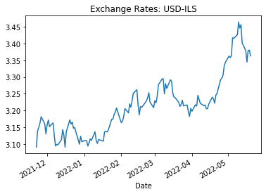
Line Chart¶

Now, let’s try to better see and and possibly explorate, the results we just recieved.

First, few actions needs to be done in prior.

import matplotlib.pyplot as plt

usd_to_ils_rates = (
    pd
    .read_html('https://www.exchange-rates.org/history/ILS/USD/T')
    [0]
    .rename(columns = {0 : 'Date', 1: 'Day', 2 : 'Rate', 3 : 'Notes'})
#     .query('Rate.str.len() < 20')
    .assign(Rate = lambda x : x.Rate.str.replace('[^\d\.]','',regex=True).astype(float))
    .assign(Date = lambda x : pd.to_datetime(x.Date))
    .set_index('Date')
)
usd_to_ils_rates

	Day	Rate	Notes
Date
2022-05-20	Friday	3.36283	USD ILS rate for 5/20/2022
2022-05-19	Thursday	3.38042	USD ILS rate for 5/19/2022
2022-05-18	Wednesday	3.37941	USD ILS rate for 5/18/2022
2022-05-17	Tuesday	3.34471	USD ILS rate for 5/17/2022
2022-05-16	Monday	3.37882	USD ILS rate for 5/16/2022
...	...	...	...
2021-11-26	Friday	3.18176	USD ILS rate for 11/26/2021
2021-11-25	Thursday	3.16222	USD ILS rate for 11/25/2021
2021-11-24	Wednesday	3.14962	USD ILS rate for 11/24/2021
2021-11-23	Tuesday	3.13881	USD ILS rate for 11/23/2021
2021-11-22	Monday	3.09072	USD ILS rate for 11/22/2021

130 rows × 3 columns

(
    usd_to_ils_rates
    ['Rate']
    .plot(title='Exchange Rates: USD-ILS')
);

../_images/08.02_Currency_analysis_38_0.png

Scatter Plot¶

Now let’s try something else, to demonstrate the differences between the days.

(
    usd_to_ils_rates
    .plot
    .scatter(
        x='Day',
        y='Rate',
        c='Red',
        title='Exchange Rates: USD-ILS across the week days'
    )
);

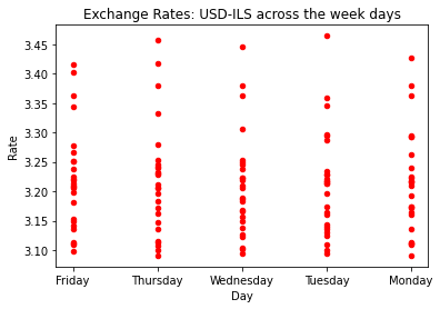
../_images/08.02_Currency_analysis_40_0.png

Something here looks odd. it appears there are less trading ‘Sundays’, which could be the reason for our former result.
Let’s check it.

(
    usd_to_ils_rates
    .groupby('Day')
    ['Rate']
    .count()
)

Day
Friday       26
Monday       26
Thursday     26
Tuesday      26
Wednesday    26
Name: Rate, dtype: int64

Yep, totally true. therefore, let’s check for the all the other days excluding Sunday.
Filtering the Dataframe to exclude Sundays.

(
    usd_to_ils_rates
    .query('Day != "Sunday"')
    .plot
    .scatter(
        x='Day',
        y='Rate',
        c='Green',
        title='Exchange Rates: USD-ILS across the working days'
    )
);

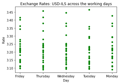
../_images/08.02_Currency_analysis_44_0.png

And based on the most lower points, we can now see that the lowest days occurs in the mid-of-the-week days.

Analyze Across Weeks using Groupby¶

Another cool way to possible be able to better identifiy the aforementioned trend, check the max & min weekly rate, and on which day did it happen.

First, let’s set up our data in a way that will allow us to analyze it.

And by a grouped table, which will show the day of each week which the highest, and later the lowest rate occured on.

(
     usd_to_ils_rates
     .assign(Week = usd_to_ils_rates.index.week)
     .groupby(['Week'])
     ['Day', 'Rate']
     .max()
     .style
     .background_gradient(cmap='summer', subset=['Rate'])
)

	Day	Rate
Week
1	Wednesday	3.115250
2	Wednesday	3.136660
3	Wednesday	3.140750
4	Wednesday	3.207520
5	Wednesday	3.206050
6	Wednesday	3.251370
7	Wednesday	3.262140
8	Wednesday	3.253240
9	Wednesday	3.276830
10	Wednesday	3.295400
11	Wednesday	3.291900
12	Wednesday	3.230900
13	Wednesday	3.216810
14	Wednesday	3.245360
15	Wednesday	3.218350
16	Wednesday	3.251140
17	Wednesday	3.343850
18	Wednesday	3.417140
19	Wednesday	3.464200
20	Wednesday	3.380420
47	Wednesday	3.181760
48	Wednesday	3.171570
49	Wednesday	3.163360
50	Wednesday	3.143060
51	Wednesday	3.172170
52	Wednesday	3.123020

(
     usd_to_ils_rates
     .assign(Week = usd_to_ils_rates.index.week)
     .groupby(['Week'])
     ['Day', 'Rate']
     .min()
     .style
     .background_gradient(cmap='summer', subset=['Rate'])
)

	Day	Rate
Week
1	Friday	3.094070
2	Friday	3.101660
3	Friday	3.108650
4	Friday	3.174190
5	Friday	3.163880
6	Friday	3.193020
7	Friday	3.187010
8	Friday	3.223520
9	Friday	3.208720
10	Friday	3.250110
11	Friday	3.238470
12	Friday	3.212440
13	Friday	3.182330
14	Friday	3.213450
15	Friday	3.205370
16	Friday	3.221920
17	Friday	3.292740
18	Friday	3.358250
19	Friday	3.401920
20	Friday	3.344710
47	Friday	3.090720
48	Friday	3.130300
49	Friday	3.094200
50	Friday	3.090750
51	Friday	3.147230
52	Friday	3.099640

Analysis conclusion¶

And here is the answer for our question - which days are the best day to conduct a currency conversion between USD and ILS to maximize your profits: Wednsday for USD to ILS and Friday to ILS to USD

From Excel to Pandas

Currency Rate Analysis

Contents