Adding New Columns
Contents
Adding New Columns
In the second chapter we will learn how to add new columns to the tables based on a set of functions. This is similar to the Functions that are available in Excel with =FUNC(A1)

We will start with loading a csv file that is hosted in data.world on the “Median Value Per Sq ft per zip code in the US”
import pandas as pd
us_median_sq_ft_value = (
    pd
    .read_csv('https://query.data.world/s/xrfy7fb7oq55gpzh6bvs6jtonv32lk')
)
us_median_sq_ft_value.head()
| RegionID | RegionName | City | State | Metro | CountyName | SizeRank | 1996-04 | 1996-05 | 1996-06 | ... | 2016-12 | 2017-01 | 2017-02 | 2017-03 | 2017-04 | 2017-05 | 2017-06 | 2017-07 | 2017-08 | 2017-09 | |
|---|---|---|---|---|---|---|---|---|---|---|---|---|---|---|---|---|---|---|---|---|---|
| 0 | 61639 | 10025 | New York | NY | New York | New York | 1 | NaN | NaN | NaN | ... | 1306.0 | 1290 | 1277 | 1272 | 1271 | 1277 | 1281 | 1279 | 1274 | 1270 |
| 1 | 84654 | 60657 | Chicago | IL | Chicago | Cook | 2 | 134.0 | 134.0 | 133.0 | ... | 291.0 | 294 | 296 | 295 | 293 | 294 | 294 | 294 | 294 | 295 |
| 2 | 61637 | 10023 | New York | NY | New York | New York | 3 | NaN | NaN | NaN | ... | 1602.0 | 1597 | 1580 | 1567 | 1569 | 1570 | 1560 | 1543 | 1529 | 1521 |
| 3 | 84616 | 60614 | Chicago | IL | Chicago | Cook | 4 | 149.0 | 150.0 | 150.0 | ... | 330.0 | 333 | 333 | 331 | 330 | 330 | 329 | 328 | 329 | 329 |
| 4 | 93144 | 79936 | El Paso | TX | El Paso | El Paso | 5 | 50.0 | 51.0 | 50.0 | ... | 81.0 | 81 | 81 | 81 | 81 | 81 | 82 | 82 | 82 | 82 |
5 rows × 265 columns
Constant Value
The simplest way to add a column is to put a constant value. Since we know that this data is only for USA we can add a column with the value USA to a new column called country. We will be able to later merge this table with data from other countries and then this new column will be useful.
For setting a value in a column we will use the assign function of Pandas. You will need to scroll all the way to the right of the output to see the new country column.
(
    us_median_sq_ft_value
    .assign(country="USA")
)
| RegionID | RegionName | City | State | Metro | CountyName | SizeRank | 1996-04 | 1996-05 | 1996-06 | ... | 2017-01 | 2017-02 | 2017-03 | 2017-04 | 2017-05 | 2017-06 | 2017-07 | 2017-08 | 2017-09 | country | |
|---|---|---|---|---|---|---|---|---|---|---|---|---|---|---|---|---|---|---|---|---|---|
| 0 | 61639 | 10025 | New York | NY | New York | New York | 1 | NaN | NaN | NaN | ... | 1290 | 1277 | 1272 | 1271 | 1277 | 1281 | 1279 | 1274 | 1270 | USA |
| 1 | 84654 | 60657 | Chicago | IL | Chicago | Cook | 2 | 134.0 | 134.0 | 133.0 | ... | 294 | 296 | 295 | 293 | 294 | 294 | 294 | 294 | 295 | USA |
| 2 | 61637 | 10023 | New York | NY | New York | New York | 3 | NaN | NaN | NaN | ... | 1597 | 1580 | 1567 | 1569 | 1570 | 1560 | 1543 | 1529 | 1521 | USA |
| 3 | 84616 | 60614 | Chicago | IL | Chicago | Cook | 4 | 149.0 | 150.0 | 150.0 | ... | 333 | 333 | 331 | 330 | 330 | 329 | 328 | 329 | 329 | USA |
| 4 | 93144 | 79936 | El Paso | TX | El Paso | El Paso | 5 | 50.0 | 51.0 | 50.0 | ... | 81 | 81 | 81 | 81 | 81 | 82 | 82 | 82 | 82 | USA |
| ... | ... | ... | ... | ... | ... | ... | ... | ... | ... | ... | ... | ... | ... | ... | ... | ... | ... | ... | ... | ... | ... |
| 14750 | 73940 | 36564 | Fairhope | AL | Daphne | Baldwin | 14751 | NaN | NaN | NaN | ... | 230 | 238 | 243 | 245 | 244 | 245 | 246 | 244 | 240 | USA |
| 14751 | 59107 | 3293 | Woodstock | NH | Claremont | Grafton | 14752 | 58.0 | 59.0 | 61.0 | ... | 129 | 129 | 128 | 129 | 130 | 130 | 130 | 130 | 131 | USA |
| 14752 | 82396 | 55713 | Buhl | MN | Duluth | Saint Louis | 14753 | NaN | NaN | NaN | ... | 72 | 73 | 74 | 74 | 73 | 73 | 74 | 77 | 79 | USA |
| 14753 | 66881 | 21405 | Annapolis | MD | Baltimore | Anne Arundel | 14754 | 146.0 | 149.0 | 151.0 | ... | 470 | 462 | 457 | 457 | 455 | 454 | 455 | 458 | 460 | USA |
| 14754 | 94815 | 85220 | Apache Junction | AZ | Phoenix | Pinal | 14755 | NaN | NaN | NaN | ... | 117 | 119 | 119 | 119 | 120 | 121 | 122 | 124 | 124 | USA |
14755 rows × 266 columns
Excel Functions Equivalent
Most of the functions that you are used to use in Excel have a direct Equivalent in Pands. We will try a few of them in the following examples. We will only look at the City column in the dataset.
For example: =TRIM('cell for trimming') can be replaced by strip.
We will:
Take only the City column from the table
Add a column that strips spaces from around the string (str) of the City column
Show the head (first 5 lines) of the new sub-table
(
    us_median_sq_ft_value[['City']]
    .assign(trimmed = us_median_sq_ft_value.City.str.strip())
    .head()
)
| City | trimmed | |
|---|---|---|
| 0 | New York | New York |
| 1 | Chicago | Chicago |
| 2 | New York | New York |
| 3 | Chicago | Chicago |
| 4 | El Paso | El Paso |
or to remove spaces between words, you will need to run ‘Find and Replace’ option in Excel and in Pandas we can use the replace function:
Take only the City column from the table
Add a column that is removes every space (‘ ‘) from the string of the City column
Show the head of the new sub-table
(
    us_median_sq_ft_value[['City']]
    .assign(no_space = us_median_sq_ft_value.City.str.replace(' ',''))
    .head()
)
| City | no_space | |
|---|---|---|
| 0 | New York | NewYork |
| 1 | Chicago | Chicago |
| 2 | New York | NewYork |
| 3 | Chicago | Chicago |
| 4 | El Paso | ElPaso |
More Textual Functions
Another commonly used Excel functions are LEFT and RIGHT (=LEFT(Cell, number of digits)). In Pandas, we can use the ‘:’, which is used for until or from:
Take only the City column from the table
Add a column that takes the first 5 characters (=LEFT) from the string of the City column
Add a column that takes the last 5 characters (=RIGHT) from the string of the City column
Show the head of the new sub-table
(
    us_median_sq_ft_value[['City']]
    .assign(city_left = us_median_sq_ft_value.City.str[:5]) # until the 5th character
    .assign(city_right = us_median_sq_ft_value.City.str[-5:]) # from the 5th characters from the end (=right)
    .head()
)
| City | city_left | city_right | |
|---|---|---|---|
| 0 | New York | New Y | York |
| 1 | Chicago | Chica | icago |
| 2 | New York | New Y | York |
| 3 | Chicago | Chica | icago |
| 4 | El Paso | El Pa | Paso |
Using Lambda
Lambda is a bit confusing at first glance, however, it is used to define a the function that we want to apply on a each row or columns of the table. For example, let’s define two new columns: one that is calculating the quantile of the region compare to all the regions, and one that is checking if the state is one of [‘NY’,’NJ’]
We will focus only on the State and the last month in the data and add the two new columns to it.
Take only the State and the values of the last period columns from the table
Add a column that checks if the State is either ‘NY’ or ‘NJ’
Add a column that calculates the ratio of the average price of the row to the maximum price (quantile)
(
    us_median_sq_ft_value[['State','2017-09']]
    .assign(is_NY_or_NJ=lambda x : x.State.isin(['NY','NJ']))
    .assign(last_quantile=lambda x : x['2017-09']/max(x['2017-09']))
)
| State | 2017-09 | is_NY_or_NJ | last_quantile | |
|---|---|---|---|---|
| 0 | NY | 1270 | True | 0.702434 |
| 1 | IL | 295 | False | 0.163164 |
| 2 | NY | 1521 | True | 0.841261 |
| 3 | IL | 329 | False | 0.181969 |
| 4 | TX | 82 | False | 0.045354 |
| ... | ... | ... | ... | ... |
| 14750 | AL | 240 | False | 0.132743 |
| 14751 | NH | 131 | False | 0.072456 |
| 14752 | MN | 79 | False | 0.043695 |
| 14753 | MD | 460 | False | 0.254425 |
| 14754 | AZ | 124 | False | 0.068584 |
14755 rows × 4 columns
Multiple Data Sources
We can do a more complicated analysis that is based on additional external sources. For example, we want to calculate the differences between red states and blue states. We can then ask various questions regarding the impacts or correlation between the house prices and the election results and voting patterns.
First we will load data regarding the voting in various states across the years. A quick internet search finds an interesting table in the following Wikipedia page. Since there are multiple tables on that page, we can filter them using the match option, and using the word Year as the filter.
Read the HTML tables in the wikipedia entry on the topic of red and blue states
retrive on the ones that have the word ‘Year’
red_blue_states_wikipedia_entry = 'https://en.wikipedia.org/wiki/Red_states_and_blue_states'
wikipedia_page_tables = (
    pd
    .read_html(
        red_blue_states_wikipedia_entry,
        match='Year'
    )
)
As we saw in the loading data from web site, the list can includes multiple tables. However, we filtered it and only have one table, and we can access it with the [0] modifier.
red_blue_states = wikipedia_page_tables[0]
red_blue_states.head()
| Year | 1972 | 1976 | 1980 | 1984 | 1988 | 1992 | 1996 | 2000 | 2004 | 2008 | 2012 | 2016 | 2020 | |
|---|---|---|---|---|---|---|---|---|---|---|---|---|---|---|
| Democratic Republican (lighter shading indicates win ≤5%) Winner received plurality of the vote but did not receive an outright majority of the popular vote Winner did not receive a plurality of the vote and lost the popular vote Winner chosen by the House of Representatives Electoral votes invalidated | Democratic Republican (lighter shading indicates win ≤5%) Winner received plurality of the vote but did not receive an outright majority of the popular vote Winner did not receive a plurality of the vote and lost the popular vote Winner chosen by the House of Representatives Electoral votes invalidated | Democratic Republican (lighter shading indicates win ≤5%) Winner received plurality of the vote but did not receive an outright majority of the popular vote Winner did not receive a plurality of the vote and lost the popular vote Winner chosen by the House of Representatives Electoral votes invalidated | Democratic Republican (lighter shading indicates win ≤5%) Winner received plurality of the vote but did not receive an outright majority of the popular vote Winner did not receive a plurality of the vote and lost the popular vote Winner chosen by the House of Representatives Electoral votes invalidated | Democratic Republican (lighter shading indicates win ≤5%) Winner received plurality of the vote but did not receive an outright majority of the popular vote Winner did not receive a plurality of the vote and lost the popular vote Winner chosen by the House of Representatives Electoral votes invalidated | Democratic Republican (lighter shading indicates win ≤5%) Winner received plurality of the vote but did not receive an outright majority of the popular vote Winner did not receive a plurality of the vote and lost the popular vote Winner chosen by the House of Representatives Electoral votes invalidated | Democratic Republican (lighter shading indicates win ≤5%) Winner received plurality of the vote but did not receive an outright majority of the popular vote Winner did not receive a plurality of the vote and lost the popular vote Winner chosen by the House of Representatives Electoral votes invalidated | Democratic Republican (lighter shading indicates win ≤5%) Winner received plurality of the vote but did not receive an outright majority of the popular vote Winner did not receive a plurality of the vote and lost the popular vote Winner chosen by the House of Representatives Electoral votes invalidated | Democratic Republican (lighter shading indicates win ≤5%) Winner received plurality of the vote but did not receive an outright majority of the popular vote Winner did not receive a plurality of the vote and lost the popular vote Winner chosen by the House of Representatives Electoral votes invalidated | Democratic Republican (lighter shading indicates win ≤5%) Winner received plurality of the vote but did not receive an outright majority of the popular vote Winner did not receive a plurality of the vote and lost the popular vote Winner chosen by the House of Representatives Electoral votes invalidated | Democratic Republican (lighter shading indicates win ≤5%) Winner received plurality of the vote but did not receive an outright majority of the popular vote Winner did not receive a plurality of the vote and lost the popular vote Winner chosen by the House of Representatives Electoral votes invalidated | Democratic Republican (lighter shading indicates win ≤5%) Winner received plurality of the vote but did not receive an outright majority of the popular vote Winner did not receive a plurality of the vote and lost the popular vote Winner chosen by the House of Representatives Electoral votes invalidated | Democratic Republican (lighter shading indicates win ≤5%) Winner received plurality of the vote but did not receive an outright majority of the popular vote Winner did not receive a plurality of the vote and lost the popular vote Winner chosen by the House of Representatives Electoral votes invalidated | Democratic Republican (lighter shading indicates win ≤5%) Winner received plurality of the vote but did not receive an outright majority of the popular vote Winner did not receive a plurality of the vote and lost the popular vote Winner chosen by the House of Representatives Electoral votes invalidated | |
| 0 | Democratic candidate | George McGovern | Jimmy Carter | Jimmy Carter | Walter Mondale | Michael Dukakis | Bill Clinton | Bill Clinton | Al Gore | John Kerry | Barack Obama | Barack Obama | Hillary Clinton | Joe Biden |
| 1 | Republican candidate | Richard Nixon | Gerald Ford | Ronald Reagan | Ronald Reagan | George H. W. Bush | George H. W. Bush | Bob Dole | George W. Bush | George W. Bush | John McCain | Mitt Romney | Donald Trump | Donald Trump |
| 2 | National popular vote | Nixon | Carter | Reagan | Reagan | Bush | Clinton | Clinton | Gore | Bush | Obama | Obama | Clinton | Biden |
| 3 | Alabama | Nixon | Carter | Reagan | Reagan | Bush | Bush | Dole | Bush | Bush | McCain | Romney | Trump | Trump |
| 4 | Alaska | Nixon | Ford | Reagan | Reagan | Bush | Bush | Dole | Bush | Bush | McCain | Romney | Trump | Trump |
We will start with creating a new list of states that voted for a specific candidate in a specific electio. First, let’s use Trump in the 2016 elections.
We are using here a few new functions such as rename, query and iloc, which we will discuss in more details in the next sections.
red_candidate = 'Trump'
We will:
Take the large table of the multiple elections results
Remove the complicated multi level header from the table (droplevel)
Filter to only states that have the name of the red candidate, we defined above, in the column of the election year (2020, for example). Note, we need to surround the name of the column with ` as it starts with a number
Take only the first column from the result table, which holds the name of the state (iloc[:,0]).
red_states_2020 = (
    red_blue_states
    .droplevel(1, axis=1)
    .query("`2020` == @red_candidate")
    .iloc[:,0]
)
red_states_2020
3            Alabama
4             Alaska
6           Arkansas
12           Florida
15             Idaho
17           Indiana
18              Iowa
19            Kansas
20          Kentucky
21         Louisiana
29       Mississippi
30          Missouri
31           Montana
39    North Carolina
40      North Dakota
41              Ohio
42          Oklahoma
46    South Carolina
47      South Dakota
48         Tennessee
49             Texas
50              Utah
54     West Virginia
56           Wyoming
Name: Year, dtype: object
Now that we have the list of the red states of 2020, we need to match them to the states that we have in our house prices data set. We see that we have to match the short version in the data set with the long version in the red state list.
We will use a another option to create a data frame using a Dictionary. It is not hard to find a list of mapping of states names and abbreviations.
us_state_abbrev = {
    'Alabama': 'AL',
    'Alaska': 'AK',
    'American Samoa': 'AS',
    'Arizona': 'AZ',
    'Arkansas': 'AR',
    'California': 'CA',
    'Colorado': 'CO',
    'Connecticut': 'CT',
    'Delaware': 'DE',
    'District of Columbia': 'DC',
    'Florida': 'FL',
    'Georgia': 'GA',
    'Guam': 'GU',
    'Hawaii': 'HI',
    'Idaho': 'ID',
    'Illinois': 'IL',
    'Indiana': 'IN',
    'Iowa': 'IA',
    'Kansas': 'KS',
    'Kentucky': 'KY',
    'Louisiana': 'LA',
    'Maine': 'ME',
    'Maryland': 'MD',
    'Massachusetts': 'MA',
    'Michigan': 'MI',
    'Minnesota': 'MN',
    'Mississippi': 'MS',
    'Missouri': 'MO',
    'Montana': 'MT',
    'Nebraska': 'NE',
    'Nevada': 'NV',
    'New Hampshire': 'NH',
    'New Jersey': 'NJ',
    'New Mexico': 'NM',
    'New York': 'NY',
    'North Carolina': 'NC',
    'North Dakota': 'ND',
    'Northern Mariana Islands':'MP',
    'Ohio': 'OH',
    'Oklahoma': 'OK',
    'Oregon': 'OR',
    'Pennsylvania': 'PA',
    'Puerto Rico': 'PR',
    'Rhode Island': 'RI',
    'South Carolina': 'SC',
    'South Dakota': 'SD',
    'Tennessee': 'TN',
    'Texas': 'TX',
    'Utah': 'UT',
    'Vermont': 'VT',
    'Virgin Islands': 'VI',
    'Virginia': 'VA',
    'Washington': 'WA',
    'West Virginia': 'WV',
    'Wisconsin': 'WI',
    'Wyoming': 'WY'
}
and we can use the dictionary to create a table (DataFrame) from it:
Create a new dataframe table
Using the dictionary of the us state abbreviation above
with row for each entry
and name the column of the value ‘Abbreviation’
us_state_abbrev_df = (
    pd
    .DataFrame
    .from_dict(us_state_abbrev,
                orient='index',
                columns=['Abbreviation'])
)
Before we continue, we can keep this table as file to be used in future analyses. We could also create this file in Excel and load it as we will do in the future with this file.
us_state_abbrev_df.to_csv('../data/us_state_abbrev.csv')
Next, we will:
Start with the abbreviation list of all the US states
Take only the ones that also appear in the list of red states in the 2020 election
Take all the rows left, and the index column (country name) with the abbreviation column
red_state_abbrev = (
    us_state_abbrev_df
    .loc[red_states_2020]
    .loc[:,'Abbreviation']
)
red_state_abbrev
Alabama           AL
Alaska            AK
Arkansas          AR
Florida           FL
Idaho             ID
Indiana           IN
Iowa              IA
Kansas            KS
Kentucky          KY
Louisiana         LA
Mississippi       MS
Missouri          MO
Montana           MT
North Carolina    NC
North Dakota      ND
Ohio              OH
Oklahoma          OK
South Carolina    SC
South Dakota      SD
Tennessee         TN
Texas             TX
Utah              UT
West Virginia     WV
Wyoming           WY
Name: Abbreviation, dtype: object
Finally:
Start with the table of the median value of sqr feet per zip code
Add a new column (is_red) that checks if the State in each row is in the list of red states that we calculated above.
Create two groups for red and blue states and the a value in the last period in the table (September 2017)
Calculate the average (mean) price for each of the two groups
Plot the two values
Title the graph with “Average square feet value between blue and red states”
(
    us_median_sq_ft_value
    .assign(is_red=lambda x : x.State.isin(red_state_abbrev))
    .groupby('is_red')['2017-09']
    .mean()
    .plot
    .bar(title="Average square feet value between blue and red states")
);
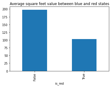
We can now see that the average value of square feet in the blue states (is_red = False) is about twice the average of red states (is_red = True)