Reading Data from External API
Contents
Reading Data from External API
Often you want to add external data to your analysis. External data can be retrieved from API (Application Programable Interface) that is provided by various services such as CRM (Customer Relationship Management) systems. You can import HTML directly into Excel using “Import”.
In this notebook, we will learn how to use pandas from_dict to load data from these external API

Loading API data
We will load a few tables from simple API as well as complex ones
import warnings
warnings.filterwarnings('ignore')
import pandas as pd
import numpy as np
Loading from simple API
If you have a simple API with no authentication, you can pass the URL of the requests library that we used in our previous toturial for loading HTML
For this excercise we will use the API of the Wikipedia page views. We will use it to test the idea that people who are thinking to buy stocks, are going to the wikipedia page of that stock, and therefore, if we see an increase in the views of a page, we will see an increase in the price of that share.
We will check the format of the API call from the technical page. We see the we need to plug the name of stock ticker, and we will use the f-string syntax that is replacing the {page} (or any other variable in curly brackets) with the value of the variable (for example, AMZN).
page = 'AMZN'

header = {
  "User-Agent": "Mozilla/5.0 (X11; Linux x86_64) AppleWebKit/537.36 (KHTML, like Gecko) Chrome/50.0.2661.75 Safari/537.36",
  "X-Requested-With": "XMLHttpRequest"
}

page_views_api_url = f'https://wikimedia.org/api/rest_v1/metrics/pageviews/per-article/en.wikipedia/all-access/all-agents/{page}/daily/2020030100/2020033000'

import requests
response = requests.get(page_views_api_url, headers=header)
response
<Response [200]>
We can use two methods to extract the data that we want from the JSON format. The first is using json_normalize and the second is using from_dict
df = (
    pd
    .json_normalize(
        response.json(),
        'items'
        )
)
df.head(5)
| project | article | granularity | timestamp | access | agent | views | |
|---|---|---|---|---|---|---|---|
| 0 | en.wikipedia | AMZN | daily | 2020030100 | all-access | all-agents | 2 |
| 1 | en.wikipedia | AMZN | daily | 2020030200 | all-access | all-agents | 6 |
| 2 | en.wikipedia | AMZN | daily | 2020030300 | all-access | all-agents | 16 |
| 3 | en.wikipedia | AMZN | daily | 2020030400 | all-access | all-agents | 1 |
| 4 | en.wikipedia | AMZN | daily | 2020030500 | all-access | all-agents | 1 |
page_view_data = (
    requests
    .get(page_views_api_url, headers=header)
    .json()['items']
)
page_views_table = (
    pd
    .DataFrame
    .from_dict(page_view_data)
)
page_views_table.head(5)
| project | article | granularity | timestamp | access | agent | views | |
|---|---|---|---|---|---|---|---|
| 0 | en.wikipedia | AMZN | daily | 2020030100 | all-access | all-agents | 2 |
| 1 | en.wikipedia | AMZN | daily | 2020030200 | all-access | all-agents | 6 |
| 2 | en.wikipedia | AMZN | daily | 2020030300 | all-access | all-agents | 16 |
| 3 | en.wikipedia | AMZN | daily | 2020030400 | all-access | all-agents | 1 |
| 4 | en.wikipedia | AMZN | daily | 2020030500 | all-access | all-agents | 1 |
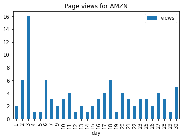
Simple Data Visualization
Start with the page view table from the previous API call
Convert the timestamp column to date time format using the %Y%m%d%H format
Extract the day of the month from the above timestamp
Plot the results
as bar chart with the day of the month as x and the number of views as y
and title the graph as ‘Page views for …’ with the name of the page
(
    page_views_table
    .assign(timestamp = lambda x: pd.to_datetime(x.timestamp, format='%Y%m%d%H', errors='coerce'))
    .assign(day = lambda x: x.timestamp.dt.day)
    .plot
    .bar(
        x='day', y='views',
        title=f'Page views for {page}'
    )
);
Loading the page views of all NASDAQ 100
We saw in the previous section how to load the values of a table from Wikipeia (or other HTML pages). Let’s use it now to load all the NASDAQ 100 index companies to compare their page views.
%pip install lxml
Requirement already satisfied: lxml in /opt/hostedtoolcache/Python/3.7.13/x64/lib/python3.7/site-packages (4.8.0)
WARNING: There was an error checking the latest version of pip.
Note: you may need to restart the kernel to use updated packages.
nasdaq_100_wikipedia_entry = 'https://en.wikipedia.org/wiki/NASDAQ-100'
nasdaq_100_tickers = (
    pd
    .read_html(
        nasdaq_100_wikipedia_entry,
        match='Ticker'
    )
)
nasdaq_100_tickers[0]
| Company | Ticker | GICS Sector | GICS Sub-Industry | |
|---|---|---|---|---|
| 0 | Activision Blizzard | ATVI | Communication Services | Interactive Home Entertainment |
| 1 | Adobe | ADBE | Information Technology | Application Software |
| 2 | ADP | ADP | Information Technology | Data Processing & Outsourced Services |
| 3 | Airbnb | ABNB | Consumer Discretionary | Internet & Direct Marketing Retail |
| 4 | Align | ALGN | Health Care | Health Care Supplies |
| ... | ... | ... | ... | ... |
| 97 | Walgreens Boots Alliance | WBA | Consumer Staples | Drug Retail |
| 98 | Workday | WDAY | Information Technology | Application Software |
| 99 | Xcel Energy | XEL | Utilities | Multi-Utilities |
| 100 | Zoom | ZM | Information Technology | Application Software |
| 101 | Zscaler | ZS | Information Technology | Application Software |
102 rows × 4 columns
Now we want to get all the views of each company on our list. We will define a simple function that will get the name of the company and return the views of this company’s page.
Generate the URL of the wikipedia page view using the name of the company
Load the API response from above URL
Parse the JSON format of the response using the key ‘items’
Return the newly create dataframe or an empty data frame if failed
def get_views(company):
    company_page_url = f'https://wikimedia.org/api/rest_v1/metrics/pageviews/per-article/en.wikipedia/all-access/all-agents/{company.iat[0,0]}/daily/2020090100/2020093000'
    response = requests.get(company_page_url, headers=header)
    try:
        df = (
            pd
            .json_normalize(
                response.json(),
                'items'
            )
        )
    except:
        df = pd.DataFrame()

    return df
Now we can apply the function above on each of the row from the nasdaq 100 tickets list:
Start with the first table from the nasdaq 100 list above
Group the ticker by the company name (in case we have multiple ticker to a company)
Apply the get view function on each of the company names and concat all the data frames together
nasdaq_100_views = (
    nasdaq_100_tickers[0]
    .head(2)
    .groupby('Company')[['Company']]
    .apply(get_views)
)
nasdaq_100_views
| project | article | granularity | timestamp | access | agent | views | ||
|---|---|---|---|---|---|---|---|---|
| Company | ||||||||
| Activision Blizzard | 0 | en.wikipedia | Activision_Blizzard | daily | 2020090100 | all-access | all-agents | 1437 |
| 1 | en.wikipedia | Activision_Blizzard | daily | 2020090200 | all-access | all-agents | 1715 | |
| 2 | en.wikipedia | Activision_Blizzard | daily | 2020090300 | all-access | all-agents | 1989 | |
| 3 | en.wikipedia | Activision_Blizzard | daily | 2020090400 | all-access | all-agents | 1628 | |
| 4 | en.wikipedia | Activision_Blizzard | daily | 2020090500 | all-access | all-agents | 1260 | |
| 5 | en.wikipedia | Activision_Blizzard | daily | 2020090600 | all-access | all-agents | 1253 | |
| 6 | en.wikipedia | Activision_Blizzard | daily | 2020090700 | all-access | all-agents | 1218 | |
| 7 | en.wikipedia | Activision_Blizzard | daily | 2020090800 | all-access | all-agents | 1331 | |
| 8 | en.wikipedia | Activision_Blizzard | daily | 2020090900 | all-access | all-agents | 1537 | |
| 9 | en.wikipedia | Activision_Blizzard | daily | 2020091000 | all-access | all-agents | 1431 | |
| 10 | en.wikipedia | Activision_Blizzard | daily | 2020091100 | all-access | all-agents | 1352 | |
| 11 | en.wikipedia | Activision_Blizzard | daily | 2020091200 | all-access | all-agents | 1042 | |
| 12 | en.wikipedia | Activision_Blizzard | daily | 2020091300 | all-access | all-agents | 1066 | |
| 13 | en.wikipedia | Activision_Blizzard | daily | 2020091400 | all-access | all-agents | 1327 | |
| 14 | en.wikipedia | Activision_Blizzard | daily | 2020091500 | all-access | all-agents | 1346 | |
| 15 | en.wikipedia | Activision_Blizzard | daily | 2020091600 | all-access | all-agents | 1267 | |
| 16 | en.wikipedia | Activision_Blizzard | daily | 2020091700 | all-access | all-agents | 1289 | |
| 17 | en.wikipedia | Activision_Blizzard | daily | 2020091800 | all-access | all-agents | 1241 | |
| 18 | en.wikipedia | Activision_Blizzard | daily | 2020091900 | all-access | all-agents | 1117 | |
| 19 | en.wikipedia | Activision_Blizzard | daily | 2020092000 | all-access | all-agents | 1137 | |
| 20 | en.wikipedia | Activision_Blizzard | daily | 2020092100 | all-access | all-agents | 4108 | |
| 21 | en.wikipedia | Activision_Blizzard | daily | 2020092200 | all-access | all-agents | 3319 | |
| 22 | en.wikipedia | Activision_Blizzard | daily | 2020092300 | all-access | all-agents | 2992 | |
| 23 | en.wikipedia | Activision_Blizzard | daily | 2020092400 | all-access | all-agents | 2312 | |
| 24 | en.wikipedia | Activision_Blizzard | daily | 2020092500 | all-access | all-agents | 1806 | |
| 25 | en.wikipedia | Activision_Blizzard | daily | 2020092600 | all-access | all-agents | 1557 | |
| 26 | en.wikipedia | Activision_Blizzard | daily | 2020092700 | all-access | all-agents | 1549 | |
| 27 | en.wikipedia | Activision_Blizzard | daily | 2020092800 | all-access | all-agents | 1564 | |
| 28 | en.wikipedia | Activision_Blizzard | daily | 2020092900 | all-access | all-agents | 1585 | |
| 29 | en.wikipedia | Activision_Blizzard | daily | 2020093000 | all-access | all-agents | 1703 | |
| Adobe | 0 | en.wikipedia | Adobe | daily | 2020090100 | all-access | all-agents | 2003 |
| 1 | en.wikipedia | Adobe | daily | 2020090200 | all-access | all-agents | 886 | |
| 2 | en.wikipedia | Adobe | daily | 2020090300 | all-access | all-agents | 844 | |
| 3 | en.wikipedia | Adobe | daily | 2020090400 | all-access | all-agents | 874 | |
| 4 | en.wikipedia | Adobe | daily | 2020090500 | all-access | all-agents | 708 | |
| 5 | en.wikipedia | Adobe | daily | 2020090600 | all-access | all-agents | 663 | |
| 6 | en.wikipedia | Adobe | daily | 2020090700 | all-access | all-agents | 795 | |
| 7 | en.wikipedia | Adobe | daily | 2020090800 | all-access | all-agents | 827 | |
| 8 | en.wikipedia | Adobe | daily | 2020090900 | all-access | all-agents | 754 | |
| 9 | en.wikipedia | Adobe | daily | 2020091000 | all-access | all-agents | 1080 | |
| 10 | en.wikipedia | Adobe | daily | 2020091100 | all-access | all-agents | 697 | |
| 11 | en.wikipedia | Adobe | daily | 2020091200 | all-access | all-agents | 679 | |
| 12 | en.wikipedia | Adobe | daily | 2020091300 | all-access | all-agents | 755 | |
| 13 | en.wikipedia | Adobe | daily | 2020091400 | all-access | all-agents | 806 | |
| 14 | en.wikipedia | Adobe | daily | 2020091500 | all-access | all-agents | 719 | |
| 15 | en.wikipedia | Adobe | daily | 2020091600 | all-access | all-agents | 850 | |
| 16 | en.wikipedia | Adobe | daily | 2020091700 | all-access | all-agents | 778 | |
| 17 | en.wikipedia | Adobe | daily | 2020091800 | all-access | all-agents | 779 | |
| 18 | en.wikipedia | Adobe | daily | 2020091900 | all-access | all-agents | 642 | |
| 19 | en.wikipedia | Adobe | daily | 2020092000 | all-access | all-agents | 863 | |
| 20 | en.wikipedia | Adobe | daily | 2020092100 | all-access | all-agents | 843 | |
| 21 | en.wikipedia | Adobe | daily | 2020092200 | all-access | all-agents | 775 | |
| 22 | en.wikipedia | Adobe | daily | 2020092300 | all-access | all-agents | 750 | |
| 23 | en.wikipedia | Adobe | daily | 2020092400 | all-access | all-agents | 784 | |
| 24 | en.wikipedia | Adobe | daily | 2020092500 | all-access | all-agents | 659 | |
| 25 | en.wikipedia | Adobe | daily | 2020092600 | all-access | all-agents | 717 | |
| 26 | en.wikipedia | Adobe | daily | 2020092700 | all-access | all-agents | 634 | |
| 27 | en.wikipedia | Adobe | daily | 2020092800 | all-access | all-agents | 740 | |
| 28 | en.wikipedia | Adobe | daily | 2020092900 | all-access | all-agents | 993 | |
| 29 | en.wikipedia | Adobe | daily | 2020093000 | all-access | all-agents | 832 |
We see that we have more than 2000 rows in the concatenated dataframe where each line is a view of a company in a specific day in the range of September 2020.
Let’s look on one of the companies (for example, Lululemon Atheletica)
nasdaq_100_views.loc['Activision Blizzard']
| project | article | granularity | timestamp | access | agent | views | |
|---|---|---|---|---|---|---|---|
| 0 | en.wikipedia | Activision_Blizzard | daily | 2020090100 | all-access | all-agents | 1437 |
| 1 | en.wikipedia | Activision_Blizzard | daily | 2020090200 | all-access | all-agents | 1715 |
| 2 | en.wikipedia | Activision_Blizzard | daily | 2020090300 | all-access | all-agents | 1989 |
| 3 | en.wikipedia | Activision_Blizzard | daily | 2020090400 | all-access | all-agents | 1628 |
| 4 | en.wikipedia | Activision_Blizzard | daily | 2020090500 | all-access | all-agents | 1260 |
| 5 | en.wikipedia | Activision_Blizzard | daily | 2020090600 | all-access | all-agents | 1253 |
| 6 | en.wikipedia | Activision_Blizzard | daily | 2020090700 | all-access | all-agents | 1218 |
| 7 | en.wikipedia | Activision_Blizzard | daily | 2020090800 | all-access | all-agents | 1331 |
| 8 | en.wikipedia | Activision_Blizzard | daily | 2020090900 | all-access | all-agents | 1537 |
| 9 | en.wikipedia | Activision_Blizzard | daily | 2020091000 | all-access | all-agents | 1431 |
| 10 | en.wikipedia | Activision_Blizzard | daily | 2020091100 | all-access | all-agents | 1352 |
| 11 | en.wikipedia | Activision_Blizzard | daily | 2020091200 | all-access | all-agents | 1042 |
| 12 | en.wikipedia | Activision_Blizzard | daily | 2020091300 | all-access | all-agents | 1066 |
| 13 | en.wikipedia | Activision_Blizzard | daily | 2020091400 | all-access | all-agents | 1327 |
| 14 | en.wikipedia | Activision_Blizzard | daily | 2020091500 | all-access | all-agents | 1346 |
| 15 | en.wikipedia | Activision_Blizzard | daily | 2020091600 | all-access | all-agents | 1267 |
| 16 | en.wikipedia | Activision_Blizzard | daily | 2020091700 | all-access | all-agents | 1289 |
| 17 | en.wikipedia | Activision_Blizzard | daily | 2020091800 | all-access | all-agents | 1241 |
| 18 | en.wikipedia | Activision_Blizzard | daily | 2020091900 | all-access | all-agents | 1117 |
| 19 | en.wikipedia | Activision_Blizzard | daily | 2020092000 | all-access | all-agents | 1137 |
| 20 | en.wikipedia | Activision_Blizzard | daily | 2020092100 | all-access | all-agents | 4108 |
| 21 | en.wikipedia | Activision_Blizzard | daily | 2020092200 | all-access | all-agents | 3319 |
| 22 | en.wikipedia | Activision_Blizzard | daily | 2020092300 | all-access | all-agents | 2992 |
| 23 | en.wikipedia | Activision_Blizzard | daily | 2020092400 | all-access | all-agents | 2312 |
| 24 | en.wikipedia | Activision_Blizzard | daily | 2020092500 | all-access | all-agents | 1806 |
| 25 | en.wikipedia | Activision_Blizzard | daily | 2020092600 | all-access | all-agents | 1557 |
| 26 | en.wikipedia | Activision_Blizzard | daily | 2020092700 | all-access | all-agents | 1549 |
| 27 | en.wikipedia | Activision_Blizzard | daily | 2020092800 | all-access | all-agents | 1564 |
| 28 | en.wikipedia | Activision_Blizzard | daily | 2020092900 | all-access | all-agents | 1585 |
| 29 | en.wikipedia | Activision_Blizzard | daily | 2020093000 | all-access | all-agents | 1703 |
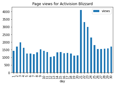
Start with the page view table of all the nasdaq 100
Filter to include only the Lululemon Athletica views
Convert the timestamp column to date time format using the %Y%m%d%H format
Extract the day of the month from the above timestamp
Plot the results
as bar chart with the day of the month as x and the number of views as y
and title the graph as ‘Page views for …’ with the name of the focused company
focused_company = 'Activision Blizzard'
(
    nasdaq_100_views
    .loc[focused_company]
    .assign(timestamp=lambda x: pd.to_datetime(x.timestamp, format='%Y%m%d%H', errors='coerce'))
    .assign(day = lambda x: x.timestamp.dt.day)
    .plot
    .bar(
        x='day', y='views',
        title=f'Page views for {focused_company}'
    )
);
Loading from complex API
Many times API are more complex, nevertheless, we can still extract the relevant data.
Let’s get some stock data from alphavantage.co
This web service is providing useful investment information using an API, however, like many other API providers, it requires an API key to identify the request (and sometimes chanrge for it).
To allow usage of secrets such as the API key for the service call, we will use a simple mechanism using .env file that each user should create and update with their private keys.
Once we have the module to handle secrets installed, we can import it to the notebook and use it. You can get your free API key from alphavantage.co. Next time you will execute the cell and the whole notebook, the API key will be retrieved from the local file.
pip install python-dotenv
Requirement already satisfied: python-dotenv in /opt/hostedtoolcache/Python/3.7.13/x64/lib/python3.7/site-packages (0.20.0)
WARNING: There was an error checking the latest version of pip.
Note: you may need to restart the kernel to use updated packages.
import os
from dotenv import load_dotenv
load_dotenv()

ALPHAVANTAGE_API_KEY = os.getenv("ALPHAVANTAGE_API_KEY")
From the API documentation we can learn how to extract time-series stock information of a specific symbol. Let’s use Amazon (AMZN) for example.
symbol = 'AMZN'

request_url = f'https://www.alphavantage.co/query?function=TIME_SERIES_INTRADAY&symbol={symbol}&interval=1min&apikey={ALPHAVANTAGE_API_KEY}'
df = (
    pd
    .read_json(request_url)
)
df
| Meta Data | Time Series (1min) | |
|---|---|---|
| 1. Information | Intraday (1min) open, high, low, close prices ... | NaN |
| 2. Symbol | AMZN | NaN |
| 3. Last Refreshed | 2022-05-20 19:59:00 | NaN |
| 4. Interval | 1min | NaN |
| 5. Output Size | Compact | NaN |
| ... | ... | ... |
| 2022-05-20 15:07:00 | NaN | {'1. open': '2108.8392', '2. high': '2111.6600... |
| 2022-05-20 15:06:00 | NaN | {'1. open': '2111.4100', '2. high': '2111.4100... |
| 2022-05-20 15:05:00 | NaN | {'1. open': '2111.1683', '2. high': '2111.1683... |
| 2022-05-20 15:04:00 | NaN | {'1. open': '2113.0875', '2. high': '2114.8200... |
| 2022-05-20 15:03:00 | NaN | {'1. open': '2117.0000', '2. high': '2117.0100... |
106 rows × 2 columns
Extracting the relevant data
We see that the data that we are looking for (open, close, high and low prices and volume in each minute) is available in a column of the dataframe table. We will filter the table to include only the rows with the prices data and split it to separated columns.
Start with the dataframe table that was returned from the API call
Rename the long ‘Time Series…’ column name to short ‘ts’
Filter out (using query) all the rows where ‘ts’ column has no value (null)
Filter (using loc) only the ‘ts’ column
Parse each value in the column as a series of key-value pairs and create a column for each pair
json_series = (
    df
    .rename(columns={'Time Series (1min)':'ts'})
    .query('ts.notnull()')
    .loc[:,'ts']
    .apply(pd.Series)
)
json_series
| 1. open | 2. high | 3. low | 4. close | 5. volume | |
|---|---|---|---|---|---|
| 2022-05-20 19:59:00 | 2157.0000 | 2157.0000 | 2157.0000 | 2157.0000 | 463 |
| 2022-05-20 19:55:00 | 2157.0000 | 2157.0000 | 2157.0000 | 2157.0000 | 227 |
| 2022-05-20 19:45:00 | 2157.1000 | 2157.1000 | 2157.1000 | 2157.1000 | 529 |
| 2022-05-20 18:43:00 | 2154.4000 | 2154.4000 | 2154.4000 | 2154.4000 | 435 |
| 2022-05-20 18:36:00 | 2151.8200 | 2151.8200 | 2151.8200 | 2151.8200 | 134 |
| ... | ... | ... | ... | ... | ... |
| 2022-05-20 15:07:00 | 2108.8392 | 2111.6600 | 2108.7900 | 2109.9900 | 8308 |
| 2022-05-20 15:06:00 | 2111.4100 | 2111.4100 | 2108.5600 | 2109.3198 | 4978 |
| 2022-05-20 15:05:00 | 2111.1683 | 2111.1683 | 2107.8600 | 2108.1201 | 9070 |
| 2022-05-20 15:04:00 | 2113.0875 | 2114.8200 | 2110.0200 | 2111.6524 | 7870 |
| 2022-05-20 15:03:00 | 2117.0000 | 2117.0100 | 2112.5700 | 2112.6300 | 13826 |
100 rows × 5 columns
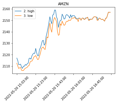
Quick Visualization
Now that we have the prices from the API we can plot them.
Start with the parsed data table above
Convert the values to numeric form (astype(‘float’))
Slice the table to include only the high and low values (iloc)
Reverse the order of the time-series to be from oldest to newest (iloc[::-1])
Plot the data
with the title of the ticker
and with 45° rotation.
(
    json_series
    .filter(['2. high','3. low'])
    .astype('float')
    .iloc[::-1]
    .plot(
        title=symbol,
        rot=45
    )
)
<AxesSubplot:title={'center':'AMZN'}>