Loading Data Files (CSV or XLSX)¶

In the first chapter we will learn how to load data into Pandas DataFrames. We will load multile formats of data sources including CSV files, Excel files, tables from web sites, tables in Databases, etc.

You can review the official Pandas documentation about reading and writing data, or you can follow the simple examples here with real life examples.

To make the notebooks cleaner and easier to read we will suppress warnings. Bad practice, however, OK for a tutorial.

import warnings
warnings.filterwarnings('ignore')

%pip install pandas matplotlib

Requirement already satisfied: pandas in /opt/hostedtoolcache/Python/3.7.13/x64/lib/python3.7/site-packages (1.3.5)
Requirement already satisfied: matplotlib in /opt/hostedtoolcache/Python/3.7.13/x64/lib/python3.7/site-packages (3.5.2)

Requirement already satisfied: pytz>=2017.3 in /opt/hostedtoolcache/Python/3.7.13/x64/lib/python3.7/site-packages (from pandas) (2022.1)
Requirement already satisfied: python-dateutil>=2.7.3 in /opt/hostedtoolcache/Python/3.7.13/x64/lib/python3.7/site-packages (from pandas) (2.8.2)
Requirement already satisfied: numpy>=1.17.3 in /opt/hostedtoolcache/Python/3.7.13/x64/lib/python3.7/site-packages (from pandas) (1.21.6)
Requirement already satisfied: pillow>=6.2.0 in /opt/hostedtoolcache/Python/3.7.13/x64/lib/python3.7/site-packages (from matplotlib) (9.1.1)
Requirement already satisfied: pyparsing>=2.2.1 in /opt/hostedtoolcache/Python/3.7.13/x64/lib/python3.7/site-packages (from matplotlib) (3.0.9)
Requirement already satisfied: kiwisolver>=1.0.1 in /opt/hostedtoolcache/Python/3.7.13/x64/lib/python3.7/site-packages (from matplotlib) (1.4.2)
Requirement already satisfied: cycler>=0.10 in /opt/hostedtoolcache/Python/3.7.13/x64/lib/python3.7/site-packages (from matplotlib) (0.11.0)
Requirement already satisfied: packaging>=20.0 in /opt/hostedtoolcache/Python/3.7.13/x64/lib/python3.7/site-packages (from matplotlib) (21.3)
Requirement already satisfied: fonttools>=4.22.0 in /opt/hostedtoolcache/Python/3.7.13/x64/lib/python3.7/site-packages (from matplotlib) (4.33.3)

Requirement already satisfied: typing-extensions in /opt/hostedtoolcache/Python/3.7.13/x64/lib/python3.7/site-packages (from kiwisolver>=1.0.1->matplotlib) (4.2.0)
Requirement already satisfied: six>=1.5 in /opt/hostedtoolcache/Python/3.7.13/x64/lib/python3.7/site-packages (from python-dateutil>=2.7.3->pandas) (1.16.0)

WARNING: There was an error checking the latest version of pip.

Note: you may need to restart the kernel to use updated packages.

Loading CSV file¶

The comma-separated-values (CSV) format is one of the simplest and pupolar way to share (small) data. You can save an Excel files as CSV and it is the default format of many bulk download of data from databases and other sources.

import pandas as pd
import numpy as np
import matplotlib

The first example is using data file about permits for restaurants in NY city. It was downloaded from the open data web site data.world, and we will use the read_csv option with default values.

Create a new table
from reading a CSV file in the local file system

table_df = (
    pd
    .read_csv('../data/open_restaurant_applications_1.csv')
)

Once we loaded the data into the table DataFrame, we can browse parts of the data and its statistics.

Let’s start with browsing the head of the data.

table_df.head()

	objectid	globalid	seating_interest_sidewalk_roadway_both	restaurant_name	legal_business_name	doing_business_as_dba	bulding_number	street	borough	postcode	...	time_of_submission	latitude	longitude	community_board	council_district	census_tract	bin	bbl	nta	location
0	32	ae5914d4-6080-4144-8634-98ca22b215de	sidewalk	Arbuz Cafe	Arbuz Cafe NY inc.	Arbuz Cafe NY inc.	1706	Sheepshead Bay Rd	Brooklyn	11235	...	2020-06-19	40.585724	-73.951767	315.0	48.0	606.0	3343289.0	3.087700e+09	Sheepshead Bay-Gerritsen Beach-Manhattan Beach	POINT(-73.951767 40.585724)
1	33	81a2bad2-5bdc-49ed-8bb6-9dc3f9798732	roadway	Nerai	Koureli Restaurant Group Inc	Nerai	55	East 54th Street	Manhattan	10022	...	2020-06-19	40.760117	-73.973162	105.0	4.0	102.0	1035748.0	1.012900e+09	Midtown-Midtown South	POINT(-73.973162 40.760117)
2	34	b4bcb3a5-e2f7-4069-8c3b-21f47f051a63	roadway	Hill Country	Hill Country New York, LLC	Hill Country	30	West 26th	Manhattan	10010	...	2020-06-19	NaN	NaN	NaN	NaN	NaN	NaN	NaN	NaN	NaN
3	35	a1054682-ff93-4b07-8f99-daa2a7b0daaf	both	Sundays Well	Two Bridge Tavern LLC	Sundays Well	360	3rd Ave	Manhattan	10016	...	2020-06-19	40.740892	-73.981657	106.0	2.0	68.0	1018142.0	1.008820e+09	Gramercy	POINT(-73.981657 40.740892)
4	36	1dd1f4e5-3e2c-4522-89e4-b3f4fc802436	roadway	Le Baba Cool, Inc	Le Baba Cool, Inc	Le Baba Cool, Inc	64	Lafayette AVe	Brooklyn	11217	...	2020-06-19	40.687102	-73.975365	302.0	35.0	35.0	3059298.0	3.021160e+09	Fort Greene	POINT(-73.975365 40.687102)

5 rows × 36 columns

As you can see, it is only showing part of the rows and parts of the columns.

If we want to understand what are the columns of the table, we can

use the info function.

table_df.info()

<class 'pandas.core.frame.DataFrame'>
RangeIndex: 7939 entries, 0 to 7938
Data columns (total 36 columns):
 #   Column                                  Non-Null Count  Dtype  
---  ------                                  --------------  -----  
 objectid                                7939 non-null   int64  
 globalid                                7939 non-null   object 
 seating_interest_sidewalk_roadway_both  7939 non-null   object 
 restaurant_name                         7939 non-null   object 
 legal_business_name                     7938 non-null   object 
 doing_business_as_dba                   7929 non-null   object 
 bulding_number                          7939 non-null   object 
 street                                  7939 non-null   object 
 borough                                 7939 non-null   object 
 postcode                                7939 non-null   int64  
business_address                        7939 non-null   object 
food_service_establishment_permit       7935 non-null   object 
sidewalk_dimensions_length              7120 non-null   float64
sidewalk_dimensions_width               7120 non-null   float64
sidewalk_dimensions_area                7120 non-null   float64
roadway_dimensions_length               5080 non-null   float64
roadway_dimensions_width                5080 non-null   float64
roadway_dimensions_area                 5080 non-null   float64
approved_for_sidewalk_seating           7939 non-null   object 
approved_for_roadway_seating            7939 non-null   object 
qualify_alcohol                         7939 non-null   object 
sla_serial_number                       5774 non-null   object 
sla_license_type                        5774 non-null   object 
landmark_district_or_building           7939 non-null   object 
landmarkdistrict_terms                  1210 non-null   object 
healthcompliance_terms                  7939 non-null   object 
time_of_submission                      7939 non-null   object 
latitude                                6943 non-null   float64
longitude                               6943 non-null   float64
community_board                         6943 non-null   float64
council_district                        6943 non-null   float64
census_tract                            6943 non-null   float64
bin                                     6888 non-null   float64
bbl                                     6888 non-null   float64
nta                                     6943 non-null   object 
location                                6943 non-null   object 
dtypes: float64(13), int64(2), object(21)
memory usage: 2.2+ MB

Next, we want to some statistics on the various numeric values. with describe we can see how many values do we have in each numeric column and some statistics such as average, minimum, maximum and their quantiles.

table_df.describe()

	objectid	postcode	sidewalk_dimensions_length	sidewalk_dimensions_width	sidewalk_dimensions_area	roadway_dimensions_length	roadway_dimensions_width	roadway_dimensions_area	latitude	longitude	community_board	council_district	census_tract	bin	bbl
count	7939.000000	7939.000000	7120.000000	7120.000000	7120.000000	5080.000000	5080.000000	5080.000000	6943.000000	6943.000000	6943.000000	6943.000000	6943.000000	6.888000e+03	6.888000e+03
mean	4006.485452	10619.992442	34.319101	10.602247	410.681882	31.530709	8.590945	280.760236	40.732316	-73.952988	231.494167	17.970906	3241.251476	2.332593e+06	2.277429e+09
std	2297.885878	1091.934677	38.058425	7.241442	1109.156427	30.240655	4.384592	513.508993	0.057959	0.061280	128.857022	15.370382	13737.582279	1.329363e+06	1.296711e+09
min	32.000000	7002.000000	0.000000	0.000000	0.000000	0.000000	0.000000	0.000000	40.511019	-74.248014	101.000000	1.000000	1.000000	1.000000e+06	0.000000e+00
25%	2016.500000	10016.000000	16.000000	6.000000	120.000000	17.000000	8.000000	128.000000	40.705540	-73.990058	105.000000	3.000000	70.000000	1.026910e+06	1.008740e+09
50%	4005.000000	10454.000000	24.000000	8.000000	225.000000	24.000000	8.000000	192.000000	40.734268	-73.968501	208.000000	15.000000	151.000000	2.046050e+06	2.037640e+09
75%	5993.500000	11220.000000	40.000000	14.000000	420.000000	38.000000	8.000000	320.000000	40.761935	-73.922195	314.000000	33.000000	483.500000	3.335991e+06	3.066340e+09
max	7992.000000	91206.000000	1000.000000	50.000000	50000.000000	1000.000000	50.000000	25000.000000	40.911190	-73.702668	503.000000	51.000000	157903.000000	5.169029e+06	5.080430e+09

You can modify the percentile that are calculated for the numeric columns by setting the values that you care about.

Start with the table above
Describe the distribution of the numeric values
Add the percentile values for p10, p50 and p90

(
    table_df
    .describe(
        percentiles = [.10, .5, .90]
    )
)

	objectid	postcode	sidewalk_dimensions_length	sidewalk_dimensions_width	sidewalk_dimensions_area	roadway_dimensions_length	roadway_dimensions_width	roadway_dimensions_area	latitude	longitude	community_board	council_district	census_tract	bin	bbl
count	7939.000000	7939.000000	7120.000000	7120.000000	7120.000000	5080.000000	5080.000000	5080.000000	6943.000000	6943.000000	6943.000000	6943.000000	6943.000000	6.888000e+03	6.888000e+03
mean	4006.485452	10619.992442	34.319101	10.602247	410.681882	31.530709	8.590945	280.760236	40.732316	-73.952988	231.494167	17.970906	3241.251476	2.332593e+06	2.277429e+09
std	2297.885878	1091.934677	38.058425	7.241442	1109.156427	30.240655	4.384592	513.508993	0.057959	0.061280	128.857022	15.370382	13737.582279	1.329363e+06	1.296711e+09
min	32.000000	7002.000000	0.000000	0.000000	0.000000	0.000000	0.000000	0.000000	40.511019	-74.248014	101.000000	1.000000	1.000000	1.000000e+06	0.000000e+00
10%	825.800000	10009.000000	12.000000	4.000000	64.000000	12.000000	6.000000	96.000000	40.661594	-74.003282	102.000000	2.000000	38.000000	1.007896e+06	1.004610e+09
50%	4005.000000	10454.000000	24.000000	8.000000	225.000000	24.000000	8.000000	192.000000	40.734268	-73.968501	208.000000	15.000000	151.000000	2.046050e+06	2.037640e+09
90%	7197.200000	11369.000000	70.000000	19.000000	800.000000	60.000000	9.000000	504.000000	40.795218	-73.869113	405.000000	39.000000	2602.000000	4.087712e+06	4.030800e+09
max	7992.000000	91206.000000	1000.000000	50.000000	50000.000000	1000.000000	50.000000	25000.000000	40.911190	-73.702668	503.000000	51.000000	157903.000000	5.169029e+06	5.080430e+09

Simple data visualization¶

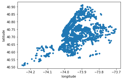
As part of the data exploration phase, you want to look at the columns, a few rows (head), column statistics (describe), data types and number of values (info). However, usually the most effective way is to visualize the data to understand it.

Start with the table above
Plot the values
as scatter plot of the data with
longitude and latitude as x-axis and y-axis, respectively.

(
    table_df
    .plot
    .scatter(
        x='longitude',
        y='latitude'
    )
);

../_images/01.01 - loading files_17_0.png

Adding new columns¶

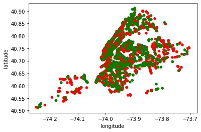
One of the most common tasks that we do when building an analysis is to add calcualted fields, based on the other columns in our table/DataFrame. We will discuss power of Pandas in adding new columns in the next sections of this guide. However, here is an example of calcuting the color of a data point, based on the value of approved_for_roadway_seating column. It will be green (g) if the value is yes, or red (r) otherwise.

Start with the loaded table data DataFrame
Add a column to color approval (approved) for road way seating as green (g)
change the color value of approved to red (r) if the value of approved_for_roadway_seating is no
Plot the result
as a scatter plot with each place
color as defined above and
in the geo location from longitude and latitude columns

(
    table_df
    .assign(approved = 'g')
    .assign(approved=lambda x : np.where(x.approved_for_roadway_seating == 'yes','g','r'))
    .plot
    .scatter(
        c='approved',
        x='longitude',
        y='latitude'
    )
);

../_images/01.01 - loading files_19_0.png

Loading Excel Files¶

You can also read files that were edited in Excel and saved in the Excel format.

If the python environment that we are using is missing part of the needed functionality, such as the ability to parse the format of the Microsoft Excel files, we need to install using the following command:

%pip install xlrd openpyxl

Requirement already satisfied: xlrd in /opt/hostedtoolcache/Python/3.7.13/x64/lib/python3.7/site-packages (2.0.1)
Requirement already satisfied: openpyxl in /opt/hostedtoolcache/Python/3.7.13/x64/lib/python3.7/site-packages (3.0.10)
Requirement already satisfied: et-xmlfile in /opt/hostedtoolcache/Python/3.7.13/x64/lib/python3.7/site-packages (from openpyxl) (1.1.0)

WARNING: There was an error checking the latest version of pip.

Note: you may need to restart the kernel to use updated packages.

Then, we can call read_excel instead of read_csv

table_df_from_excel = (
    pd
    .read_excel('../data/open_restaurant_applications.xlsx')
)

and since the data now is in the Pandas (pd) DataFrame format, all the rest of the commands are exactly the same. For example, here is the same first chart we plotted before.

(
    table_df_from_excel
    .plot
    .scatter(
        x='longitude',
        y='latitude'
    )
);

From Excel to Pandas

Loading Data Files (CSV or XLSX)

Contents

Loading Data Files (CSV or XLSX)¶

Loading CSV file¶

Simple data visualization¶

Adding new columns¶

Loading Excel Files¶