Merge/Join Tables (VLOOKUP)
Contents
Merge/Join Tables (VLOOKUP)
The merge function mimics the functionality of JOIN in SQL queries and replaces the VLOOKUP functionality in Excel. It is one of the most powerful and useful functions for dataframes in Pandas. The main idea is to:
join two (or more) dataframe table using similar keys in each of the tables.
enrich tables with loopup data
validate the match values of the key columns in the tables

import pandas as pd
Loading lookup data
For this example, we will take one of the common lookup data, zip code. The loopup is not trivial as there are a few tousands (more than 33,000 as you can see below) of values and a simple Excel file will struggle to do it efficently and quickly.
We will start with loading the loopup data from Simple Maps, which I’ve downloaded to a public S3 bucket.
url = 'https://mlguy-public.s3-eu-west-1.amazonaws.com/excel2pandas/chapter3/simplemaps_uszips_basicv1/uszips.csv'

import requests
from io import StringIO

response = requests.get(url)
response
<Response [200]>
The CSV file is read through a URL and therefore, we need to convert the text of the response to a simple string as we get when we read a local file. For that we will use the StringIO functionality as follows:
zip_lookup = (
    pd
    .read_csv(
        StringIO(
            response.text
        )
    )
)

zip_lookup
| zip | lat | lng | city | state_id | state_name | zcta | parent_zcta | population | density | county_fips | county_name | county_weights | county_names_all | county_fips_all | imprecise | military | timezone | |
|---|---|---|---|---|---|---|---|---|---|---|---|---|---|---|---|---|---|---|
| 0 | 601 | 18.18004 | -66.75218 | Adjuntas | PR | Puerto Rico | True | NaN | 17242 | 111.4 | 72001 | Adjuntas | {'72001':99.43,'72141':0.57} | Adjuntas|Utuado | 72001|72141 | False | False | America/Puerto_Rico |
| 1 | 602 | 18.36073 | -67.17517 | Aguada | PR | Puerto Rico | True | NaN | 38442 | 523.5 | 72003 | Aguada | {'72003':100} | Aguada | 72003 | False | False | America/Puerto_Rico |
| 2 | 603 | 18.45439 | -67.12202 | Aguadilla | PR | Puerto Rico | True | NaN | 48814 | 667.9 | 72005 | Aguadilla | {'72005':100} | Aguadilla | 72005 | False | False | America/Puerto_Rico |
| 3 | 606 | 18.16724 | -66.93828 | Maricao | PR | Puerto Rico | True | NaN | 6437 | 60.4 | 72093 | Maricao | {'72093':94.88,'72121':1.35,'72153':3.78} | Maricao|Yauco|Sabana Grande | 72093|72153|72121 | False | False | America/Puerto_Rico |
| 4 | 610 | 18.29032 | -67.12243 | Anasco | PR | Puerto Rico | True | NaN | 27073 | 312.0 | 72011 | Añasco | {'72003':0.55,'72011':99.45} | Añasco|Aguada | 72011|72003 | False | False | America/Puerto_Rico |
| ... | ... | ... | ... | ... | ... | ... | ... | ... | ... | ... | ... | ... | ... | ... | ... | ... | ... | ... |
| 33092 | 99923 | 55.97796 | -130.03671 | Hyder | AK | Alaska | True | NaN | 15 | 2.1 | 2198 | Prince of Wales-Hyder | {'02198':100} | Prince of Wales-Hyder | 02198 | False | False | America/Sitka |
| 33093 | 99925 | 55.55767 | -132.97627 | Klawock | AK | Alaska | True | NaN | 927 | 5.7 | 2198 | Prince of Wales-Hyder | {'02198':100} | Prince of Wales-Hyder | 02198 | False | False | America/Sitka |
| 33094 | 99926 | 55.12617 | -131.48928 | Metlakatla | AK | Alaska | True | NaN | 1635 | 4.2 | 2198 | Prince of Wales-Hyder | {'02198':100} | Prince of Wales-Hyder | 02198 | False | False | America/Metlakatla |
| 33095 | 99927 | 56.25100 | -133.37571 | Point Baker | AK | Alaska | True | NaN | 38 | 0.2 | 2198 | Prince of Wales-Hyder | {'02198':100} | Prince of Wales-Hyder | 02198 | False | False | America/Sitka |
| 33096 | 99929 | 56.36950 | -131.93648 | Wrangell | AK | Alaska | True | NaN | 2484 | 0.4 | 2275 | Wrangell | {'02275':100} | Wrangell | 02275 | False | False | America/Sitka |
33097 rows × 18 columns
Lookup Data Exploration
The table above shows us the type of data that we can get from enrichment based on the zip code, including city, state, latitude, longitude, population count and density.
We can explore the values that we have in this table, before we start to use it for enrichment.
Counting Values
The simplest aggregation function for each group is the size. How many zip codes do we have in each state?
(
    zip_lookup
    .groupby('state_name')
    .size()
)
state_name
Alabama                  642
Alaska                   238
Arizona                  405
Arkansas                 591
California              1761
Colorado                 525
Connecticut              282
Delaware                  67
District of Columbia      52
Florida                  981
Georgia                  735
Hawaii                    94
Idaho                    277
Illinois                1383
Indiana                  775
Iowa                     934
Kansas                   697
Kentucky                 767
Louisiana                515
Maine                    432
Maryland                 468
Massachusetts            537
Michigan                 986
Minnesota                884
Mississippi              423
Missouri                1022
Montana                  361
Nebraska                 581
Nevada                   175
New Hampshire            248
New Jersey               595
New Mexico               368
New York                1794
North Carolina           808
North Dakota             383
Ohio                    1195
Oklahoma                 648
Oregon                   417
Pennsylvania            1795
Puerto Rico              131
Rhode Island              77
South Carolina           424
South Dakota             371
Tennessee                628
Texas                   1935
Utah                     287
Vermont                  255
Virginia                 896
Washington               596
West Virginia            706
Wisconsin                772
Wyoming                  178
dtype: int64
Sorting Values
To sort the values is also simple with sort_value() function, and see the population size of each state (based on the zip code lookup data):
Start with the zip lookup data above
Group the row by state_name and take only the population values
Sum up all the population values for each zip code area in the state Group
Sort the states by the accumulated population value in descending order
us_population_distribution = (
    zip_lookup
    .groupby('state_name')['population']
    .sum()
    .sort_values(ascending=False)
)

us_population_distribution
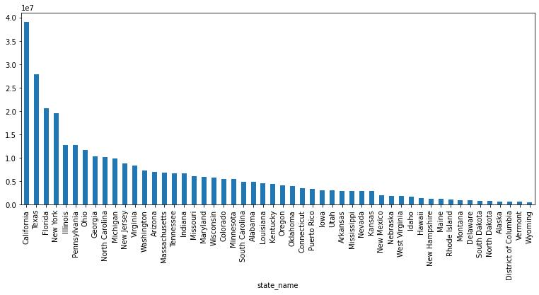
state_name
California              39140219
Texas                   27884135
Florida                 20594164
New York                19618323
Illinois                12821487
Pennsylvania            12790950
Ohio                    11639989
Georgia                 10297534
North Carolina          10155624
Michigan                 9957465
New Jersey               8881845
Virginia                 8414042
Washington               7280023
Arizona                  6949259
Massachusetts            6830133
Tennessee                6644470
Indiana                  6637220
Missouri                 6090358
Maryland                 6003435
Wisconsin                5777892
Colorado                 5531233
Minnesota                5527473
South Carolina           4955925
Alabama                  4864630
Louisiana                4663243
Kentucky                 4446667
Oregon                   4081732
Oklahoma                 3918473
Connecticut              3581504
Puerto Rico              3384779
Iowa                     3133061
Utah                     3043806
Arkansas                 2990472
Mississippi              2988710
Nevada                   2923171
Kansas                   2908448
New Mexico               2089570
Nebraska                 1904901
West Virginia            1828786
Idaho                    1687214
Hawaii                   1422019
New Hampshire            1343673
Maine                    1332721
Rhode Island             1056611
Montana                  1042359
Delaware                  949495
South Dakota              864012
North Dakota              751250
Alaska                    737979
District of Columbia      684390
Vermont                   624977
Wyoming                   582091
Name: population, dtype: int64
Visualization of the data
(
    us_population_distribution
    .plot
    .bar(figsize=(13,5))
);
Loading the main data
We will take the data about brewries in the US that we used in one of the previous lessson, and enrich it with the data from the zip codes table. We will load it from the local file after we retried the data from the API before.
breweries_data= pd.read_csv('../data/us_breweries.csv')
breweries_data.head()
| id | name | brewery_type | street | address_2 | address_3 | city | state | county_province | postal_code | country | longitude | latitude | phone | website_url | updated_at | created_at | |
|---|---|---|---|---|---|---|---|---|---|---|---|---|---|---|---|---|---|
| 0 | 2 | Avondale Brewing Co | micro | 201 41st St S | NaN | NaN | Birmingham | Alabama | NaN | 35222-1932 | United States | -86.774322 | 33.524521 | 2.057775e+09 | http://www.avondalebrewing.com | 2018-08-23T23:19:57.825Z | 2018-07-24T01:32:47.255Z |
| 1 | 44 | Trim Tab Brewing | micro | 2721 5th Ave S | NaN | NaN | Birmingham | Alabama | NaN | 35233-3401 | United States | -86.791400 | 33.512849 | 2.057031e+09 | http://www.trimtabbrewing.com | 2018-08-23T23:20:31.423Z | 2018-07-24T01:32:47.815Z |
| 2 | 46 | Yellowhammer Brewery | micro | 2600 Clinton Ave W | NaN | NaN | Huntsville | Alabama | NaN | 35805-3046 | United States | -86.593201 | 34.727752 | 2.569756e+09 | http://www.yellowhammerbrewery.com | 2018-08-23T23:20:33.102Z | 2018-07-24T01:32:47.838Z |
| 3 | 55 | Bearpaw River Brewing Co | micro | 4605 E Palmer Wasilla Hwy | NaN | NaN | Wasilla | Alaska | NaN | 99654-7679 | United States | -149.412710 | 61.575269 | NaN | http://bearpawriverbrewing.com | 2018-08-23T23:20:40.743Z | 2018-07-24T01:32:47.967Z |
| 4 | 76 | King Street Brewing Co | micro | 9050 King Street | NaN | NaN | Anchorage | Alaska | NaN | 99515 | United States | -149.879076 | 61.138489 | 9.073365e+09 | http://www.kingstreetbrewing.com | 2018-08-23T23:20:57.179Z | 2018-07-24T01:32:48.301Z |
We can see that the postal code is sometimes in the longer format (for example, 35222-1932) compare to the zip codes that we have in our lookup table (for example, 35222). We will convert them to the shorter format by taking the first 5 characters ([:5]) of the string of the postal_code column.
breweries_data_with_zip = (
    breweries_data
    .assign(zip_code = lambda x : x.postal_code.str[:5])
)
breweries_data_with_zip.head()
| id | name | brewery_type | street | address_2 | address_3 | city | state | county_province | postal_code | country | longitude | latitude | phone | website_url | updated_at | created_at | zip_code | |
|---|---|---|---|---|---|---|---|---|---|---|---|---|---|---|---|---|---|---|
| 0 | 2 | Avondale Brewing Co | micro | 201 41st St S | NaN | NaN | Birmingham | Alabama | NaN | 35222-1932 | United States | -86.774322 | 33.524521 | 2.057775e+09 | http://www.avondalebrewing.com | 2018-08-23T23:19:57.825Z | 2018-07-24T01:32:47.255Z | 35222 |
| 1 | 44 | Trim Tab Brewing | micro | 2721 5th Ave S | NaN | NaN | Birmingham | Alabama | NaN | 35233-3401 | United States | -86.791400 | 33.512849 | 2.057031e+09 | http://www.trimtabbrewing.com | 2018-08-23T23:20:31.423Z | 2018-07-24T01:32:47.815Z | 35233 |
| 2 | 46 | Yellowhammer Brewery | micro | 2600 Clinton Ave W | NaN | NaN | Huntsville | Alabama | NaN | 35805-3046 | United States | -86.593201 | 34.727752 | 2.569756e+09 | http://www.yellowhammerbrewery.com | 2018-08-23T23:20:33.102Z | 2018-07-24T01:32:47.838Z | 35805 |
| 3 | 55 | Bearpaw River Brewing Co | micro | 4605 E Palmer Wasilla Hwy | NaN | NaN | Wasilla | Alaska | NaN | 99654-7679 | United States | -149.412710 | 61.575269 | NaN | http://bearpawriverbrewing.com | 2018-08-23T23:20:40.743Z | 2018-07-24T01:32:47.967Z | 99654 |
| 4 | 76 | King Street Brewing Co | micro | 9050 King Street | NaN | NaN | Anchorage | Alaska | NaN | 99515 | United States | -149.879076 | 61.138489 | 9.073365e+09 | http://www.kingstreetbrewing.com | 2018-08-23T23:20:57.179Z | 2018-07-24T01:32:48.301Z | 99515 |
Joining the tables
The joining of the table is based on a joined key. In this case we want to use the 5-digits zip code as the lookup or join key. In the previous step with shorten the longer zip codes to the shorter 5 digits format, and now we will make sure that the lookup table also have it in the same format.
Start with the zip loopup table
Add a column zip_code that is based on the value of the column zip
Convert the numeric value into string (astype(str)),
Pad the string with zeros when the number is shorter than 5 digits (zfill(5)).
zip_lookup_as_string = (
    zip_lookup
    .assign(
        zip_code = lambda x : x.zip
        .astype(str)
        .str
        .zfill(5)
    )
)
The join itself is simple.
Start with the breweries table that you want to enrich
Join using merge with the second zip loopup table
Define the key column with the same name (zip_code), and we use it using the on argument
Lastly, we want to have all breweries, even if we don’t find the zip code in the lookup table. Therefore, we are using LEFT join using the how argument.
enriched_breweries_data = (
    breweries_data_with_zip
    .merge(
        zip_lookup_as_string,
        on='zip_code',
        how='left'
    )
)
We have now many more columns as all the columns of both tables are joined to the enriched table. We will ask the Jupyter notebook to show us all the columns by removing the default maximum number of columns to display.
In the table below we can see all the columns. If the same column name is found in both tables and it wasn’t the column that was used for the join or merge, the column of first (“left”) table will be appended with x (city_x, for example), and the column of the second (“right”) table will be appended with y (city_y, for example).
pd.set_option('display.max_columns', None)
enriched_breweries_data
| id | name | brewery_type | street | address_2 | address_3 | city_x | state | county_province | postal_code | country | longitude | latitude | phone | website_url | updated_at | created_at | zip_code | zip | lat | lng | city_y | state_id | state_name | zcta | parent_zcta | population | density | county_fips | county_name | county_weights | county_names_all | county_fips_all | imprecise | military | timezone | |
|---|---|---|---|---|---|---|---|---|---|---|---|---|---|---|---|---|---|---|---|---|---|---|---|---|---|---|---|---|---|---|---|---|---|---|---|---|
| 0 | 2 | Avondale Brewing Co | micro | 201 41st St S | NaN | NaN | Birmingham | Alabama | NaN | 35222-1932 | United States | -86.774322 | 33.524521 | 2.057775e+09 | http://www.avondalebrewing.com | 2018-08-23T23:19:57.825Z | 2018-07-24T01:32:47.255Z | 35222 | 35222.0 | 33.52409 | -86.77025 | Birmingham | AL | Alabama | True | NaN | 9033.0 | 815.8 | 1073.0 | Jefferson | {'01073':100} | Jefferson | 01073 | False | False | America/Chicago |
| 1 | 44 | Trim Tab Brewing | micro | 2721 5th Ave S | NaN | NaN | Birmingham | Alabama | NaN | 35233-3401 | United States | -86.791400 | 33.512849 | 2.057031e+09 | http://www.trimtabbrewing.com | 2018-08-23T23:20:31.423Z | 2018-07-24T01:32:47.815Z | 35233 | 35233.0 | 33.50876 | -86.80194 | Birmingham | AL | Alabama | True | NaN | 1715.0 | 300.7 | 1073.0 | Jefferson | {'01073':100} | Jefferson | 01073 | False | False | America/Chicago |
| 2 | 46 | Yellowhammer Brewery | micro | 2600 Clinton Ave W | NaN | NaN | Huntsville | Alabama | NaN | 35805-3046 | United States | -86.593201 | 34.727752 | 2.569756e+09 | http://www.yellowhammerbrewery.com | 2018-08-23T23:20:33.102Z | 2018-07-24T01:32:47.838Z | 35805 | 35805.0 | 34.70858 | -86.62125 | Huntsville | AL | Alabama | True | NaN | 21200.0 | 949.7 | 1089.0 | Madison | {'01089':100} | Madison | 01089 | False | False | America/Chicago |
| 3 | 55 | Bearpaw River Brewing Co | micro | 4605 E Palmer Wasilla Hwy | NaN | NaN | Wasilla | Alaska | NaN | 99654-7679 | United States | -149.412710 | 61.575269 | NaN | http://bearpawriverbrewing.com | 2018-08-23T23:20:40.743Z | 2018-07-24T01:32:47.967Z | 99654 | 99654.0 | 61.45483 | -149.90045 | Wasilla | AK | Alaska | True | NaN | 62135.0 | 40.4 | 2170.0 | Matanuska-Susitna | {'02170':100} | Matanuska-Susitna | 02170 | False | False | America/Anchorage |
| 4 | 76 | King Street Brewing Co | micro | 9050 King Street | NaN | NaN | Anchorage | Alaska | NaN | 99515 | United States | -149.879076 | 61.138489 | 9.073365e+09 | http://www.kingstreetbrewing.com | 2018-08-23T23:20:57.179Z | 2018-07-24T01:32:48.301Z | 99515 | 99515.0 | 61.11739 | -149.88889 | Anchorage | AK | Alaska | True | NaN | 23402.0 | 818.8 | 2020.0 | Anchorage | {'02020':100} | Anchorage | 02020 | False | False | America/Anchorage |
| ... | ... | ... | ... | ... | ... | ... | ... | ... | ... | ... | ... | ... | ... | ... | ... | ... | ... | ... | ... | ... | ... | ... | ... | ... | ... | ... | ... | ... | ... | ... | ... | ... | ... | ... | ... | ... |
| 7445 | 345 | Barrel Brothers Brewing Company | micro | 399 Business Park Ct Ste 506 | NaN | NaN | Windsor | California | NaN | 95492-6652 | United States | NaN | NaN | 7.076969e+09 | http://www.barrelbrothersbrewing.com | 2018-08-11T21:35:55.480Z | 2018-07-24T01:32:52.148Z | 95492 | 95492.0 | 38.53034 | -122.81716 | Windsor | CA | California | True | NaN | 29920.0 | 579.0 | 6097.0 | Sonoma | {'06097':100} | Sonoma | 06097 | False | False | America/Los_Angeles |
| 7446 | 352 | Bay Bridge Brewing Co | micro | 688 Marsat Ct Ste B | NaN | NaN | Chula Vista | California | NaN | 91911-4697 | United States | NaN | NaN | 6.199347e+09 | http://www.baybridgebrewing.com | 2018-08-11T21:35:55.704Z | 2018-07-24T01:32:52.238Z | 91911 | 91911.0 | 32.60738 | -117.05405 | Chula Vista | CA | California | True | NaN | 85365.0 | 2736.2 | 6073.0 | San Diego | {'06073':100} | San Diego | 06073 | False | False | America/Los_Angeles |
| 7447 | 367 | Benchmark Brewing Co | micro | 6190 Fairmount Ave Ste G | NaN | NaN | San Diego | California | NaN | 92120-3428 | United States | NaN | NaN | 6.197953e+09 | http://www.benchmarkbrewing.com | 2018-08-11T21:35:56.157Z | 2018-07-24T01:32:52.420Z | 92120 | 92120.0 | 32.79468 | -117.07114 | San Diego | CA | California | True | NaN | 29142.0 | 1501.7 | 6073.0 | San Diego | {'06073':100} | San Diego | 06073 | False | False | America/Los_Angeles |
| 7448 | 477 | Chino Valley Brewery | micro | 1609 E. Grove Ave, Unit 109 | NaN | NaN | Ontario | California | NaN | 91761-5786 | United States | NaN | NaN | 9.512917e+09 | http://www.chinovalleybrewery.com | 2018-08-11T21:35:59.331Z | 2018-07-24T01:32:53.774Z | 91761 | 91761.0 | 34.03459 | -117.59212 | Ontario | CA | California | True | NaN | 61124.0 | 754.0 | 6071.0 | San Bernardino | {'06071':100} | San Bernardino | 06071 | False | False | America/Los_Angeles |
| 7449 | 509 | Crooked Goat Brewing | micro | 120 Morris St Ste 120 | NaN | NaN | Sebastopol | California | NaN | 95472-3867 | United States | NaN | NaN | 7.078274e+09 | http://www.crookedgoatbrewing.com | 2018-08-11T21:36:00.652Z | 2018-07-24T01:32:54.205Z | 95472 | 95472.0 | 38.39817 | -122.86574 | Sebastopol | CA | California | True | NaN | 30762.0 | 157.8 | 6097.0 | Sonoma | {'06097':100} | Sonoma | 06097 | False | False | America/Los_Angeles |
7450 rows × 36 columns
Now, that we have the enriched table, we can analyze the joined data and explore the different counties across the US:
Start with the enriched breweries data above
Group the breweries by county_name
For each group add the State ID
count the number of breweries,
sum up the populations of each zip code area in each group
and calculate the average population density in the county
Sort that list by the population size
(
    enriched_breweries_data
    .groupby('county_name')
    .agg(
        state=('state_id', 'min'),
        brewry_count=('id', 'count'),
        population_sum=('population', 'sum'),
        density_average=('density', 'mean')
        )
    .sort_values(by='population_sum', ascending=False)
)
| state | brewry_count | population_sum | density_average | |
|---|---|---|---|---|
| county_name | ||||
| San Diego | CA | 154 | 6059002.0 | 1670.298052 |
| Los Angeles | CA | 126 | 4529555.0 | 2834.088095 |
| Cook | IL | 98 | 4510406.0 | 5011.613265 |
| King | WA | 117 | 3519428.0 | 2407.258120 |
| Orange | CA | 88 | 3261503.0 | 1574.422727 |
| ... | ... | ... | ... | ... |
| Clearwater | ID | 1 | 164.0 | 5.800000 |
| Koochiching | MN | 1 | 151.0 | 334.400000 |
| Harding | NM | 1 | 139.0 | 0.100000 |
| Wabasha | MN | 1 | 88.0 | 29.500000 |
| Keweenaw | MI | 1 | 87.0 | 1.000000 |
959 rows × 4 columns
We can see that san Diego is the largest county in terms of population and also a beer county with 154 different brewries in it.
Let’s change the sort key to find the counties with the most breweries
(
    enriched_breweries_data
    .groupby('county_name')
    .agg(
        state=('state_id', 'min'),
        brewry_count=('id', 'count'),
        population_sum=('population', 'sum'),
        density_average=('density', 'mean')
        )
    .sort_values(by='brewry_count', ascending=False)
)
| state | brewry_count | population_sum | density_average | |
|---|---|---|---|---|
| county_name | ||||
| San Diego | CA | 154 | 6059002.0 | 1670.298052 |
| Los Angeles | CA | 126 | 4529555.0 | 2834.088095 |
| King | WA | 117 | 3519428.0 | 2407.258120 |
| Cook | IL | 98 | 4510406.0 | 5011.613265 |
| Jefferson | AL | 93 | 1951501.0 | 770.348387 |
| ... | ... | ... | ... | ... |
| Flagler | FL | 1 | 43813.0 | 247.300000 |
| Fond du Lac | WI | 1 | 10579.0 | 37.900000 |
| Pitkin | CO | 1 | 10653.0 | 8.900000 |
| Pine | MN | 1 | 9609.0 | 21.600000 |
| Accomack | VA | 1 | 2899.0 | 58.800000 |
959 rows × 4 columns
If you remember the map of the US that we saw in the previous section, it is now more clear the Cook county in IL is likely the dark area we saw in our hexbin visualization of the data, as a dense population of breweries.
We can now ask ourselves where do we have the most brewries per population and add this column to our table
(
    enriched_breweries_data
    .groupby('county_name')
    .agg(
        state=('state_id', 'min'),
        brewry_count=('id', 'count'),
        population_sum=('population', 'sum'),
        density_average=('density', 'mean')
        )
    .assign(brewry_per_population = lambda x : x.brewry_count / x.population_sum * 1000)
    .sort_values(by='brewry_per_population', ascending=False)
)
| state | brewry_count | population_sum | density_average | brewry_per_population | |
|---|---|---|---|---|---|
| county_name | |||||
| Keweenaw | MI | 1 | 87.0 | 1.000000 | 11.494253 |
| Wabasha | MN | 1 | 88.0 | 29.500000 | 11.363636 |
| Harding | NM | 1 | 139.0 | 0.100000 | 7.194245 |
| Koochiching | MN | 1 | 151.0 | 334.400000 | 6.622517 |
| Clearwater | ID | 1 | 164.0 | 5.800000 | 6.097561 |
| ... | ... | ... | ... | ... | ... |
| Cabarrus | NC | 5 | 299927.0 | 256.800000 | 0.016671 |
| Fort Bend | TX | 6 | 371516.0 | 472.583333 | 0.016150 |
| Chesapeake | VA | 1 | 65603.0 | 155.100000 | 0.015243 |
| Guadalupe | TX | 7 | 494106.0 | 113.828571 | 0.014167 |
| Hidalgo | TX | 4 | 287487.0 | 798.050000 | 0.013914 |
959 rows × 5 columns
We can see, as it is often the case, that we have on the top and the bottom of the table counties with very few brewries. The top of the table of brewries per 1000 people is held by Keweenaw that was last on our previous table of counties by population. To avoid this, we can filter (using query) our table to counties that have more than 5 brewries.
(
    enriched_breweries_data
    .groupby('county_name')
    .agg(
        state=('state_id', 'min'),
        brewry_count=('id', 'count'),
        population_sum=('population', 'sum'),
        density_average=('density', 'mean')
        )
    .assign(brewry_per_population = lambda x : x.brewry_count / x.population_sum * 1000)
    .query("brewry_count > 5")
    .sort_values(by='brewry_per_population', ascending=False)
)
| state | brewry_count | population_sum | density_average | brewry_per_population | |
|---|---|---|---|---|---|
| county_name | |||||
| Schuyler | NY | 7 | 15117.0 | 26.285714 | 0.463055 |
| Grafton | NH | 7 | 25969.0 | 28.714286 | 0.269552 |
| Windsor | VT | 7 | 28073.0 | 36.228571 | 0.249350 |
| Waldo | ME | 7 | 28697.0 | 28.357143 | 0.243928 |
| Grand | CO | 7 | 30992.0 | 3.485714 | 0.225865 |
| ... | ... | ... | ... | ... | ... |
| St. Charles | MO | 7 | 356115.0 | 426.171429 | 0.019657 |
| Kings | CA | 30 | 1706298.0 | 14137.416667 | 0.017582 |
| Gwinnett | GA | 6 | 349573.0 | 737.716667 | 0.017164 |
| Fort Bend | TX | 6 | 371516.0 | 472.583333 | 0.016150 |
| Guadalupe | TX | 7 | 494106.0 | 113.828571 | 0.014167 |
299 rows × 5 columns
And the winner is Schuyler county in New York, with 7 brewries and a 0.46 brewry for every 1,000 people
Geographic Mapping
The merge that we did allows us now to have geo location information for all the breweries, including the ones that didn’t have it in the original data set, as we have the geo location of the zip code area.
We can also add layers on real maps using the library GeoPandas. Let’s start with installing the library to our environment.
pip install geopandas
Collecting geopandas
  Downloading geopandas-0.10.2-py2.py3-none-any.whl (1.0 MB)
?25l     ━━━━━━━━━━━━━━━━━━━━━━━━━━━━━━━━━━━━━━━━ 0.0/1.0 MB ? eta -:--:--
     ━━━━━━━━━━━━━━━━━━━━━━━━━━━━━━━━━━╺━━━━━ 0.9/1.0 MB 27.2 MB/s eta 0:00:01
     ━━━━━━━━━━━━━━━━━━━━━━━━━━━━━━━━━━━━━━━━ 1.0/1.0 MB 24.7 MB/s eta 0:00:00
?25hRequirement already satisfied: pandas>=0.25.0 in /opt/hostedtoolcache/Python/3.7.13/x64/lib/python3.7/site-packages (from geopandas) (1.3.5)
Collecting pyproj>=2.2.0
  Downloading pyproj-3.2.1-cp37-cp37m-manylinux2010_x86_64.whl (6.3 MB)
?25l     ━━━━━━━━━━━━━━━━━━━━━━━━━━━━━━━━━━━━━━━━ 0.0/6.3 MB ? eta -:--:--
━━━━━━━━━━━━━━━━━━━━━━━━━━━╸━━━━━━━━━━━━ 4.4/6.3 MB 132.0 MB/s eta 0:00:01
     ━━━━━━━━━━━━━━━━━━━━━━━━━━━━━━━━━━━━━━━╸ 6.3/6.3 MB 129.8 MB/s eta 0:00:01
     ━━━━━━━━━━━━━━━━━━━━━━━━━━━━━━━━━━━━━━━━ 6.3/6.3 MB 85.6 MB/s eta 0:00:00
?25h
Collecting shapely>=1.6
  Downloading Shapely-1.8.2-cp37-cp37m-manylinux_2_12_x86_64.manylinux2010_x86_64.whl (2.0 MB)
?25l     ━━━━━━━━━━━━━━━━━━━━━━━━━━━━━━━━━━━━━━━━ 0.0/2.0 MB ? eta -:--:--
     ━━━━━━━━━━━━━━━━━━━━━━━━━━━━━━━━━━━━━━━━ 2.0/2.0 MB 109.6 MB/s eta 0:00:00
?25h
Collecting fiona>=1.8
  Downloading Fiona-1.8.21-cp37-cp37m-manylinux2014_x86_64.whl (16.7 MB)
?25l     ━━━━━━━━━━━━━━━━━━━━━━━━━━━━━━━━━━━━━━━━ 0.0/16.7 MB ? eta -:--:--
━━━━━━━━━━━━━╸━━━━━━━━━━━━━━━━━━━━━━━━━━ 5.7/16.7 MB 173.1 MB/s eta 0:00:01
━━━━━━━━━━━━━━━━━━━━━━━━━━━╸━━━━━━━━━━━ 11.9/16.7 MB 175.4 MB/s eta 0:00:01
     ━━━━━━━━━━━━━━━━━━━━━━━━━━━━━━━━━━━━━━╸ 16.7/16.7 MB 178.2 MB/s eta 0:00:01
     ━━━━━━━━━━━━━━━━━━━━━━━━━━━━━━━━━━━━━━╸ 16.7/16.7 MB 178.2 MB/s eta 0:00:01
     ━━━━━━━━━━━━━━━━━━━━━━━━━━━━━━━━━━━━━━━━ 16.7/16.7 MB 94.9 MB/s eta 0:00:00
?25h
Collecting munch
  Downloading munch-2.5.0-py2.py3-none-any.whl (10 kB)
Requirement already satisfied: certifi in /opt/hostedtoolcache/Python/3.7.13/x64/lib/python3.7/site-packages (from fiona>=1.8->geopandas) (2022.5.18.1)
Requirement already satisfied: six>=1.7 in /opt/hostedtoolcache/Python/3.7.13/x64/lib/python3.7/site-packages (from fiona>=1.8->geopandas) (1.16.0)
Requirement already satisfied: click>=4.0 in /opt/hostedtoolcache/Python/3.7.13/x64/lib/python3.7/site-packages (from fiona>=1.8->geopandas) (8.1.3)
Requirement already satisfied: attrs>=17 in /opt/hostedtoolcache/Python/3.7.13/x64/lib/python3.7/site-packages (from fiona>=1.8->geopandas) (21.4.0)
Collecting cligj>=0.5
  Downloading cligj-0.7.2-py3-none-any.whl (7.1 kB)
Requirement already satisfied: setuptools in /opt/hostedtoolcache/Python/3.7.13/x64/lib/python3.7/site-packages (from fiona>=1.8->geopandas) (47.1.0)
Collecting click-plugins>=1.0
  Downloading click_plugins-1.1.1-py2.py3-none-any.whl (7.5 kB)
Requirement already satisfied: python-dateutil>=2.7.3 in /opt/hostedtoolcache/Python/3.7.13/x64/lib/python3.7/site-packages (from pandas>=0.25.0->geopandas) (2.8.2)
Requirement already satisfied: numpy>=1.17.3 in /opt/hostedtoolcache/Python/3.7.13/x64/lib/python3.7/site-packages (from pandas>=0.25.0->geopandas) (1.21.6)
Requirement already satisfied: pytz>=2017.3 in /opt/hostedtoolcache/Python/3.7.13/x64/lib/python3.7/site-packages (from pandas>=0.25.0->geopandas) (2022.1)
Requirement already satisfied: importlib-metadata in /opt/hostedtoolcache/Python/3.7.13/x64/lib/python3.7/site-packages (from click>=4.0->fiona>=1.8->geopandas) (4.11.4)
Requirement already satisfied: typing-extensions>=3.6.4 in /opt/hostedtoolcache/Python/3.7.13/x64/lib/python3.7/site-packages (from importlib-metadata->click>=4.0->fiona>=1.8->geopandas) (4.2.0)
Requirement already satisfied: zipp>=0.5 in /opt/hostedtoolcache/Python/3.7.13/x64/lib/python3.7/site-packages (from importlib-metadata->click>=4.0->fiona>=1.8->geopandas) (3.8.0)
Installing collected packages: shapely, pyproj, munch, cligj, click-plugins, fiona, geopandas
Successfully installed click-plugins-1.1.1 cligj-0.7.2 fiona-1.8.21 geopandas-0.10.2 munch-2.5.0 pyproj-3.2.1 shapely-1.8.2
WARNING: There was an error checking the latest version of pip.
Note: you may need to restart the kernel to use updated packages.
We also need to install a library to handle geo coordinates
pip install descartes
Collecting descartes
  Downloading descartes-1.1.0-py3-none-any.whl (5.8 kB)
Requirement already satisfied: matplotlib in /opt/hostedtoolcache/Python/3.7.13/x64/lib/python3.7/site-packages (from descartes) (3.5.2)
Requirement already satisfied: fonttools>=4.22.0 in /opt/hostedtoolcache/Python/3.7.13/x64/lib/python3.7/site-packages (from matplotlib->descartes) (4.33.3)
Requirement already satisfied: packaging>=20.0 in /opt/hostedtoolcache/Python/3.7.13/x64/lib/python3.7/site-packages (from matplotlib->descartes) (21.3)
Requirement already satisfied: cycler>=0.10 in /opt/hostedtoolcache/Python/3.7.13/x64/lib/python3.7/site-packages (from matplotlib->descartes) (0.11.0)
Requirement already satisfied: pillow>=6.2.0 in /opt/hostedtoolcache/Python/3.7.13/x64/lib/python3.7/site-packages (from matplotlib->descartes) (9.1.1)
Requirement already satisfied: numpy>=1.17 in /opt/hostedtoolcache/Python/3.7.13/x64/lib/python3.7/site-packages (from matplotlib->descartes) (1.21.6)
Requirement already satisfied: kiwisolver>=1.0.1 in /opt/hostedtoolcache/Python/3.7.13/x64/lib/python3.7/site-packages (from matplotlib->descartes) (1.4.2)
Requirement already satisfied: python-dateutil>=2.7 in /opt/hostedtoolcache/Python/3.7.13/x64/lib/python3.7/site-packages (from matplotlib->descartes) (2.8.2)
Requirement already satisfied: pyparsing>=2.2.1 in /opt/hostedtoolcache/Python/3.7.13/x64/lib/python3.7/site-packages (from matplotlib->descartes) (3.0.9)
Requirement already satisfied: typing-extensions in /opt/hostedtoolcache/Python/3.7.13/x64/lib/python3.7/site-packages (from kiwisolver>=1.0.1->matplotlib->descartes) (4.2.0)
Requirement already satisfied: six>=1.5 in /opt/hostedtoolcache/Python/3.7.13/x64/lib/python3.7/site-packages (from python-dateutil>=2.7->matplotlib->descartes) (1.16.0)
Installing collected packages: descartes
Successfully installed descartes-1.1.0
WARNING: There was an error checking the latest version of pip.
Note: you may need to restart the kernel to use updated packages.
We will import the library
import geopandas
Create a data frame that is designed for geo data
Start with the enriched breweries data above
Define the geometry of the data from
x as the longitude (lng column)
y as the latitude (lat column)
gdf = (
    geopandas
    .GeoDataFrame(
    enriched_breweries_data,
    geometry=geopandas
    .points_from_xy(
        enriched_breweries_data.lng,
        enriched_breweries_data.lat)
    )
)
Create a geo dataframe for the world map from the built-in dataset of GeoPandas library
world = (
    geopandas
    .read_file(
        geopandas
        .datasets
        .get_path('naturalearth_lowres')
    )
)
Start with the world data frame
Filter it to use only the USA parts
Focus on the geometry boundaries of the map
Plot the map
using black color
and thin lines (0.2)
Now, plot the breweries data
on the above map
using red dots
and one pixel for each
# We restrict to USA
ax = (
    world
    [world.iso_a3 == 'USA']
    ['geometry']
    .boundary
    .plot(
        color='black',
        edgecolor='black',
        linewidth=0.2
    )
)

(
    gdf
    .plot(
        ax=ax,
        color='red',
        markersize = 1
    )
);
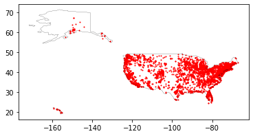
This is a good start, but we can’t really use it. Let’s make it more usable to know where is the beer hub in the US.
Create a 2D histogram based on the enriched breweries data
using x as latitude (lat column),
y as longtitude (lng column),
and 1000 bins for the histogram
Focus only on the main land using its coordinates
Then, create a smooth heat map from the histogram
import numpy as np
from scipy import ndimage

heatmap, xedges, yedges = np.histogram2d(
    enriched_breweries_data['lat'],
    enriched_breweries_data['lng'],
    bins=1000,
    range=[
        [25, 50],  # North-South extent of US
        [-125, -65]  # East-West extent of US,
    ]
)
extent = [yedges[0], yedges[-1], xedges[-1], xedges[0]]
logheatmap = np.log(heatmap)
logheatmap[np.isneginf(logheatmap)] = 0
logheatmap = ndimage.filters.gaussian_filter(logheatmap, 30, mode='nearest')  # smooth out peaks
/opt/hostedtoolcache/Python/3.7.13/x64/lib/python3.7/site-packages/ipykernel_launcher.py:14: RuntimeWarning: divide by zero encountered in log
ax = (
    world
    [world.iso_a3 == 'USA']
    ['geometry']
    .boundary
    .plot(
        color='k',
        edgecolor='black',
        linewidth=0.5
    )
)

ax.imshow(logheatmap, cmap='coolwarm', extent=extent)
ax.invert_yaxis()
ax.set(xlim=[-125, -65], ylim=[25, 50]);
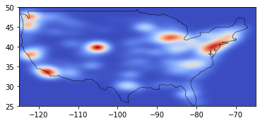
We can clearly see the hubs in San Diego, New York, Illinois, and another one in Colorado.