Date Functions
Contents
Date Functions
In the previous section we created an advanced analysis with merge and groupby and other Pandas capabilities, which are harder to do in Excel. In this section, we will check the more traditional functions that are often used in Excel spreadsheet and we will see how to use them easily in Pandas.

Date Functions
Let’s review some common functions in Excel and their replacement in Pandas
TODAY
=TODAY()
Like many of the Pandas functions, most of the arguments are optional and the default values are often as expected. For example, the time stamp and even the date depends on the timezone needed. In the next example, we will specific the optional tz value to ‘America/Chicago’:
You can see that the data includes columns such as Seasons or Functioning Day, however, we might want to calculate such columns differently.
import pandas as pd
now = (
    pd
    .Timestamp
    .today(
        tz='America/Chicago'
    )
)
now
Timestamp('2022-05-22 15:27:59.957694-0500', tz='America/Chicago')
DAY, MONTH, YEAR
We can apply all the various date functions from excel such as DAY, MINUTE, HOUR etc.
now.day, now.month, now.year
(22, 5, 2022)
DATE
we can create a date with given values such as day, month, and year
=Date(2021,1,1)
and in pandas:
new_year = (
    pd
    .Timestamp(
        year=2021,
        month=1,
        day=1
    )
)
new_year
Timestamp('2021-01-01 00:00:00')
NETWORKDAYS
A common function in business context is =NETWORKDAYS(), that calculates the number of working days between two dates. In Pandas we can use the following:
import numpy as np

(
    np
    .busday_count(
        new_year.date(),
        now.date()
    )
)
361
WORKDAY
The next useful function is =WORKDAY(NUMBER) that can be used when you want to get the date after a given number of working days
new_year = pd.Timestamp("2021-01-01")
new_year.day_name()
'Friday'
workday_100 = new_year + 100 * pd.offsets.BusinessDay()
workday_100
Timestamp('2021-05-21 00:00:00')
The one hundred working day in 2021 is May 21st.
Pandas has a wide range of options for date offsets, such as weeks, month-end, semi-month-end (15th day), querter, retail year (aka 52-53 week), and many others.
Real life example
Loading Data
As usual, let’s load a dataset to work on. We will take another dataset that is used in machine learning education, “Bike Share”. This is a data set about the demand of bike share service in Seoul. Please note that we need to modify the default encoding of read_csv from ‘UTF-8’ to ‘latin1’.
bike_share_data = (
    pd
    .read_csv(
        'https://archive.ics.uci.edu/ml/machine-learning-databases/00560/SeoulBikeData.csv',
        encoding='latin1'
    )
)
bike_share_data
| Date | Rented Bike Count | Hour | Temperature(°C) | Humidity(%) | Wind speed (m/s) | Visibility (10m) | Dew point temperature(°C) | Solar Radiation (MJ/m2) | Rainfall(mm) | Snowfall (cm) | Seasons | Holiday | Functioning Day | |
|---|---|---|---|---|---|---|---|---|---|---|---|---|---|---|
| 0 | 01/12/2017 | 254 | 0 | -5.2 | 37 | 2.2 | 2000 | -17.6 | 0.0 | 0.0 | 0.0 | Winter | No Holiday | Yes |
| 1 | 01/12/2017 | 204 | 1 | -5.5 | 38 | 0.8 | 2000 | -17.6 | 0.0 | 0.0 | 0.0 | Winter | No Holiday | Yes |
| 2 | 01/12/2017 | 173 | 2 | -6.0 | 39 | 1.0 | 2000 | -17.7 | 0.0 | 0.0 | 0.0 | Winter | No Holiday | Yes |
| 3 | 01/12/2017 | 107 | 3 | -6.2 | 40 | 0.9 | 2000 | -17.6 | 0.0 | 0.0 | 0.0 | Winter | No Holiday | Yes |
| 4 | 01/12/2017 | 78 | 4 | -6.0 | 36 | 2.3 | 2000 | -18.6 | 0.0 | 0.0 | 0.0 | Winter | No Holiday | Yes |
| ... | ... | ... | ... | ... | ... | ... | ... | ... | ... | ... | ... | ... | ... | ... |
| 8755 | 30/11/2018 | 1003 | 19 | 4.2 | 34 | 2.6 | 1894 | -10.3 | 0.0 | 0.0 | 0.0 | Autumn | No Holiday | Yes |
| 8756 | 30/11/2018 | 764 | 20 | 3.4 | 37 | 2.3 | 2000 | -9.9 | 0.0 | 0.0 | 0.0 | Autumn | No Holiday | Yes |
| 8757 | 30/11/2018 | 694 | 21 | 2.6 | 39 | 0.3 | 1968 | -9.9 | 0.0 | 0.0 | 0.0 | Autumn | No Holiday | Yes |
| 8758 | 30/11/2018 | 712 | 22 | 2.1 | 41 | 1.0 | 1859 | -9.8 | 0.0 | 0.0 | 0.0 | Autumn | No Holiday | Yes |
| 8759 | 30/11/2018 | 584 | 23 | 1.9 | 43 | 1.3 | 1909 | -9.3 | 0.0 | 0.0 | 0.0 | Autumn | No Holiday | Yes |
8760 rows × 14 columns
Date Columns Manipulations
We will start with creating a few columns based on the date column, such as day of the week and month.
Start with the table we loaded above
Make sure that the Date column is in datetime format that we see (note the day before the month)
Calculate the day-of-week (DOW) of each row (to use the built-in functions we need to access the date accessor (.dt))
Calculate the month value of each row
enriched_bike_share_data = (
    bike_share_data
    .assign(Date = pd.to_datetime(bike_share_data.Date, format='%d/%m/%Y', errors='coerce'))
    .assign(DOW = lambda x : x.Date.dt.day_name())
    .assign(month = lambda x : x.Date.dt.month)
)
enriched_bike_share_data
| Date | Rented Bike Count | Hour | Temperature(°C) | Humidity(%) | Wind speed (m/s) | Visibility (10m) | Dew point temperature(°C) | Solar Radiation (MJ/m2) | Rainfall(mm) | Snowfall (cm) | Seasons | Holiday | Functioning Day | DOW | month | |
|---|---|---|---|---|---|---|---|---|---|---|---|---|---|---|---|---|
| 0 | 2017-12-01 | 254 | 0 | -5.2 | 37 | 2.2 | 2000 | -17.6 | 0.0 | 0.0 | 0.0 | Winter | No Holiday | Yes | Friday | 12 |
| 1 | 2017-12-01 | 204 | 1 | -5.5 | 38 | 0.8 | 2000 | -17.6 | 0.0 | 0.0 | 0.0 | Winter | No Holiday | Yes | Friday | 12 |
| 2 | 2017-12-01 | 173 | 2 | -6.0 | 39 | 1.0 | 2000 | -17.7 | 0.0 | 0.0 | 0.0 | Winter | No Holiday | Yes | Friday | 12 |
| 3 | 2017-12-01 | 107 | 3 | -6.2 | 40 | 0.9 | 2000 | -17.6 | 0.0 | 0.0 | 0.0 | Winter | No Holiday | Yes | Friday | 12 |
| 4 | 2017-12-01 | 78 | 4 | -6.0 | 36 | 2.3 | 2000 | -18.6 | 0.0 | 0.0 | 0.0 | Winter | No Holiday | Yes | Friday | 12 |
| ... | ... | ... | ... | ... | ... | ... | ... | ... | ... | ... | ... | ... | ... | ... | ... | ... |
| 8755 | 2018-11-30 | 1003 | 19 | 4.2 | 34 | 2.6 | 1894 | -10.3 | 0.0 | 0.0 | 0.0 | Autumn | No Holiday | Yes | Friday | 11 |
| 8756 | 2018-11-30 | 764 | 20 | 3.4 | 37 | 2.3 | 2000 | -9.9 | 0.0 | 0.0 | 0.0 | Autumn | No Holiday | Yes | Friday | 11 |
| 8757 | 2018-11-30 | 694 | 21 | 2.6 | 39 | 0.3 | 1968 | -9.9 | 0.0 | 0.0 | 0.0 | Autumn | No Holiday | Yes | Friday | 11 |
| 8758 | 2018-11-30 | 712 | 22 | 2.1 | 41 | 1.0 | 1859 | -9.8 | 0.0 | 0.0 | 0.0 | Autumn | No Holiday | Yes | Friday | 11 |
| 8759 | 2018-11-30 | 584 | 23 | 1.9 | 43 | 1.3 | 1909 | -9.3 | 0.0 | 0.0 | 0.0 | Autumn | No Holiday | Yes | Friday | 11 |
8760 rows × 16 columns
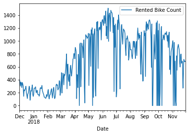
Simple Data Visulizations
Start with the enriched table above
Group the data by date column
Calculate the mean of values per each day
Plot the results with date as x and number of rented bike as y
(
    enriched_bike_share_data
    .groupby('Date')
    .mean()
    .plot(y='Rented Bike Count')
);
Start with the enriched table above
Group the data by date column
Calculate the mean of values per each day
Plot the results
with scatter plot with temp as x and number of rented bike as y
(
    enriched_bike_share_data
    .groupby('Date')
    .mean()
    .plot
    .scatter(x='Temperature(°C)', y='Rented Bike Count')
);
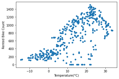
Analyzing Corrlations between the columns
Start with the enriched table above
Group the data by date column
Calculate the mean of values per each day
Calculate the correlation values between the numeric values
Take the values that are related to the first column (Rented Bike Count), skip the first two rows (self correlation, and hour column)
Add style to the output
Highlight the maximum correlation value with green background
and Highlight the minimum correlation value with red background
(
    enriched_bike_share_data
    .groupby('Date')
    .mean()
    .corr()
    .iloc[2:,[0]]
    .style
    .highlight_max(color='green')
    .highlight_min(color='red')
)
| Rented Bike Count | |
|---|---|
| Temperature(°C) | 0.699824 |
| Humidity(%) | 0.028158 |
| Wind speed (m/s) | -0.174859 |
| Visibility (10m) | 0.145376 |
| Dew point temperature(°C) | 0.602648 |
| Solar Radiation (MJ/m2) | 0.684069 |
| Rainfall(mm) | -0.214252 |
| Snowfall (cm) | -0.240836 |
| month | 0.201733 |
We can see that the higher correlation is with the temperature (the higher the temperature, the more bikes are rented), and with the Snowfall (the more snowfall, the fewer bikes are reneted), which make sense.